VCEMethods


Polynomials
In methods, we are mainly concerned with linear, quadratic and cubic polynomials. Their additive (fully expanded) forms are respectively: \[ \begin {aligned} y &=mx + c \\ y &= ax^2 + bx + c \\ y &= ax^3 + bx^2 + cx + d \end{aligned} \]
In general, a polynomial has the additive form: \[y = a_{n}\cdot x^{n} + a_{(n-1)}\cdot x^{n-1} + … + a_{0}\]
Note that the coefficient of the leading term (term where x has the highest power) must not equal 0
As indicated above, a quadratic has a leading term with degree (power) 2. Other than the full expanded form, there are two other important forms which we must be aware of - Turning point and product (intercept) forms. Respectively:
\[y = a(x-h)^2+k\]
a dilates the function and dictates whether the parabola opens upwards or downwards (more on this later).
h is the x-coordinate of the turning point.
k is the y-coordinate of the turning point.
\[y = a(x-b)(x-c)\]
a dilates the function and dictates whether the parabola opens upwards or downwards (more on this later).
(b,0) is a x-intercept.
(c,0) is a x-intercept.
A parabola is symmetric about a vertical line. When a quadratic is presented in the full expanded form:
\[y = ax^2 + bx + c\]
The axis of symmetry is:
\[x = -\frac{b}{2a}\]
This is also the x-coordinate of the turning point.
Completing the square can be quite difficult. As such, we do not recommend using this technique unless you have to.
Completing the square for \(y = ax^2+bx+c\)
| \[1\] | \[\text{Factor out } a\] \[ y = a(x^2 + \frac{b}{a}x + \frac{c}{a})\] |
| \[2\] | \[\text{Take note of the sign in front of } \frac{b}{a}x.\] |
| \[3\] |
Halve the coefficient in front of \(x\) and add or subtract it to \(x\) depending on the sign from step 2. Square this, add the constant to it and subtract the halved coefficient squared. This whole expression should be multiplied by \(a\) the coefficient which we factored out in step 1 \[y = a((x+\frac{b}{2a})^2+c- (\frac{b}{2a})^2)\] |
| \[4\] | \[\text{Add the constant terms together}\] \[y = a((x+\frac{b}{2a})^2+c-\frac{b^2}{4a^2})\] |
| \[5\] | \[ \text{Simplify the equation as required}\\ y=a(x+\frac{b}{2a})^2+ac-\frac{b^2}{4a} \] |
\[\text{Example 4.1: Convert the equation into turning point form by completing the square }\\ \begin{aligned} y &= 2x^2 -14x+24 \\ \text{ }\\ y &= 2x^2 - 14x+24 \\ &= 2(x^2 - 7x + 12) \\ &= 2((x - \frac{7}{2})^2+12-(\frac{7}{2})^2 )\\ &= 2((x - \frac{7}{2})^2+12-\frac{49}{4})\\ &= 2((x - \frac{7}{2})^2+12-\frac{49}{4})\\ &= 2((x - \frac{7}{2})^2-\frac{1}{4})\\ \end{aligned} \]
| 1 | Move all terms to one side |
| 2 | Attempt to factorise using the method above (if not possible move to step 3) and then set each factor equal to 0 and solve |
| 3 | Use the quadratic formula. (Skip if step 2 completed successfully) |
The quadratic formula allows us to find the solutions to a quadratic equation of the form: \[0 = ax^2 + bx + c\] Quadratic formula: \[x = \frac{-b \pm \sqrt{b^2-4ac}}{2a}\]
\[ \text{Example 4.2: Solve }4x^2=8x + 21 \text{ for } x\\ \text{ }\\ \text{1. Move all terms to one side}\\ 4x^2 - 8x - 21 = 0\\ \text{ }\\ \text{2. Attempt to factorise and set each factor equal to 0}\\ (2x-7)(2x+3)=0\\ 2x-7 = 0,\, 2x+3=0\\ x = \frac{7}{2},\, -\frac{3}{2}\\ \text{ }\\ \text{3. If you were unable to factorise, use the quadratic equation.}\\ \begin{aligned} x &= \frac{-(-8) \pm \sqrt{(-8)^2-4(4)(-21)}}{2\cdot4}\\ x &= \frac{8 \pm \sqrt{64+336}}{8}\\ x &= \frac{8 \pm \sqrt{400}}{8}\\ x &= \frac{8 \pm \sqrt{20}}{8}\\ x &= \frac{28}{8} , -\frac{12}{8}\\ x &= \frac{7}{2} , -\frac{3}{2}\\ \end{aligned}\\ \]
The basic shape of a quadratic is shown below.
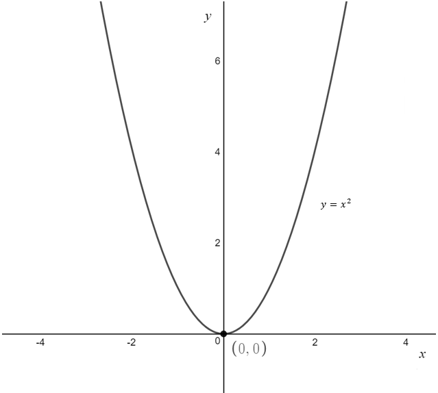
In general, unless told not to, all graphs must provide the coordinates or equations of any: x-intercepts, y-intercepts and asymptotes. The basic shape of a quadratic is shown above. There are three different ways to graph quadratics.
Method 1 - Use when provided equation in turning point form \[y = a(x-h)^2 + k\]
| 1 | Mark out the coordinate of the turning point at (h,k) |
| 2 | Substitute x = 0 into the equation and solve for y to find the y-intercept |
| 3 | Substitute y = 0 into the equation and solve for x to find the x-intercept(s) (you will need to expand the quadratic expression) |
| 4 | Connect the dots appropriately |
| 5 | Check that your parabola opens the correct way. The parabola will open upwards if a > 0 and downwards if a < 0 |
| 6 | Adjust the graph according to the domain, finding the coordinates of the endpoints if required. Label with the equation. |
Method 2 - Use when provided equation in product (intercept) form \[y = a(x-b)(x-c)\]
| 1 | Mark out the coordinates of the x-intercepts at (b,0) and (c,0) |
| 2 | Substitute x = 0 into the equation and solve for y to find the y-intercept |
| 3 | Connect the dots appropriately |
| 4 | Check that your parabola opens the correct way. The parabola will open upwards if a > 0 and downwards if a < 0. For every negative coefficient in front of a x, you will need to switch the other sign. View examples for more details. |
| 5 | Adjust the graph according to the domain, finding the coordinates of the endpoints if required. Label with the equation. |
Method 3 - Use when provided equation in additive (expanded) form \[y = ax^2+bx+c\]
| 1 | Mark out the coordinates of the y-intercepts at (0,c) |
| 2 | Substitute y = 0 into the equation and solve for x to find the x-intercept(s) (you will need to expand the quadratic expression) |
| 3 | Connect the dots appropriately. |
| 4 | Check that your parabola opens the correct way. The parabola will open upwards if a > 0 and downwards if a < 0. |
| 5 | Adjust the graph according to the domain, finding the coordinates of the endpoints if required. Label with the equation. |
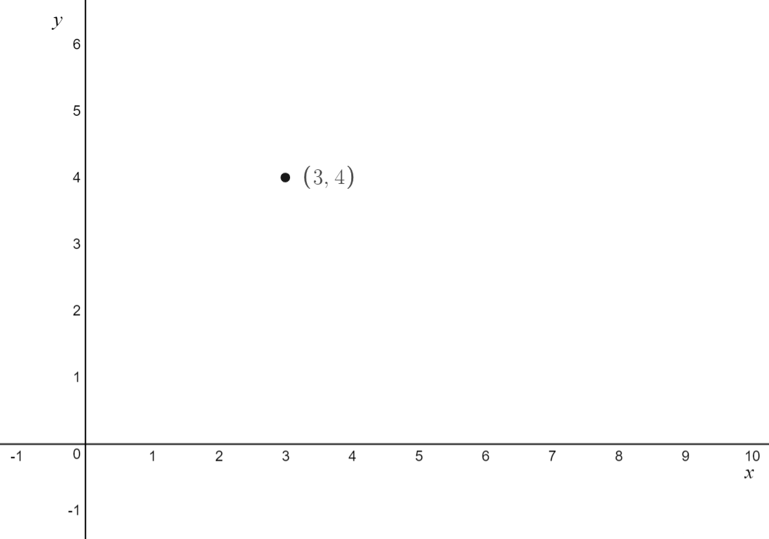
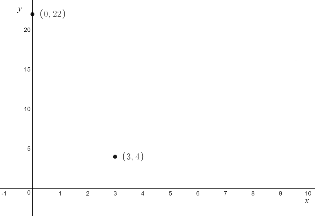
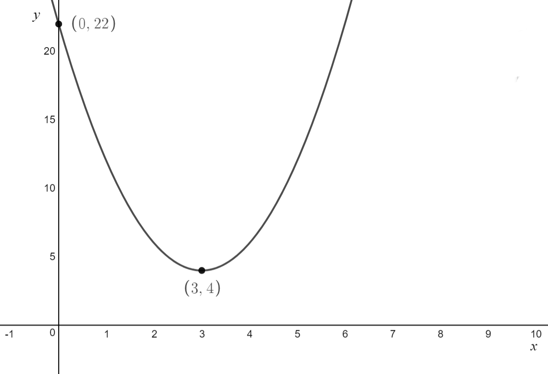
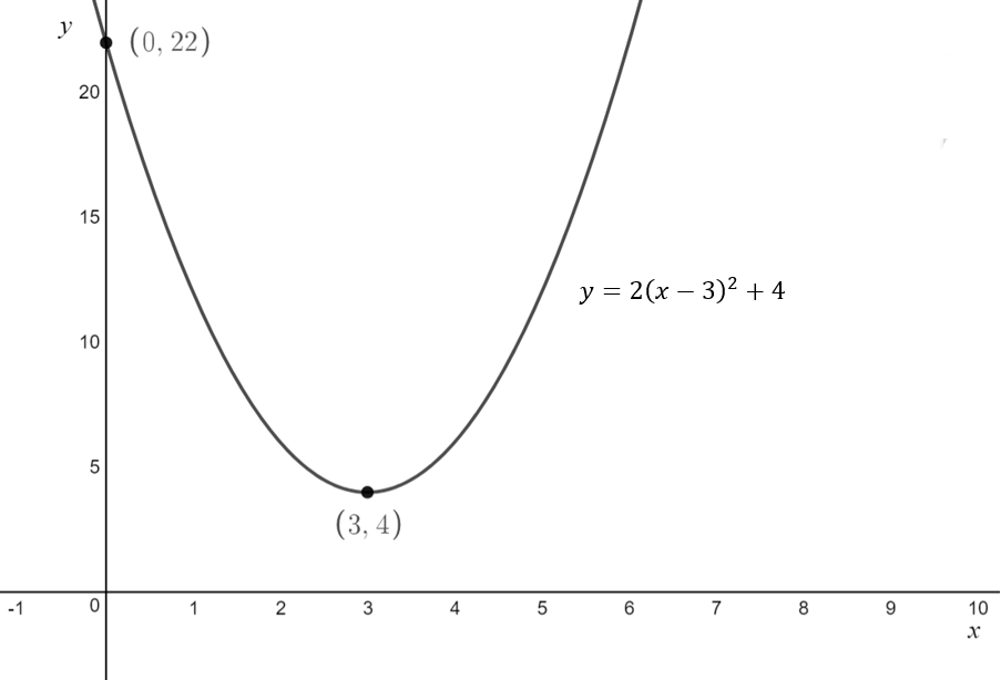
\[\text{Example 4.3: Sketch } f(x) = 2(x-3)^2+4 \\ \text{ labelling any x-intercepts, y-intercepts and turning points}\]
\[
\text{1. Mark in the turning point} \\
\text{The turning point has coordinates } (3,4)
\]
 \[
\text{ } \\
\text{2. Find the y-intercept} \\
\begin{aligned}
x&= 0\\
y&= 2(0-3)^2+4 \\
y&= 2 \cdot 9 + 4 \\
y &= 18 + 4\\
y&= 22\\
\end{aligned}\\
\text{There is a y-intercept at } (0,22)
\]
\[
\text{ } \\
\text{2. Find the y-intercept} \\
\begin{aligned}
x&= 0\\
y&= 2(0-3)^2+4 \\
y&= 2 \cdot 9 + 4 \\
y &= 18 + 4\\
y&= 22\\
\end{aligned}\\
\text{There is a y-intercept at } (0,22)
\]
 \[
\text{ } \\
\text{3. Find the x-intercepts} \\
\text{This parabola opens upwards and has a turning point} \\ \text{above the x-axis, so will not have any x intercepts}
\]
\[
\text{ } \\
\text{4. Connect the dots}
\]
\[
\text{ } \\
\text{3. Find the x-intercepts} \\
\text{This parabola opens upwards and has a turning point} \\ \text{above the x-axis, so will not have any x intercepts}
\]
\[
\text{ } \\
\text{4. Connect the dots}
\]
 \[
\text{4. Label the equation}
\]
\[
\text{4. Label the equation}
\]
 \[
\text{ } \\
\text{5. The domain is not restricted. No changes need to be made}
\]
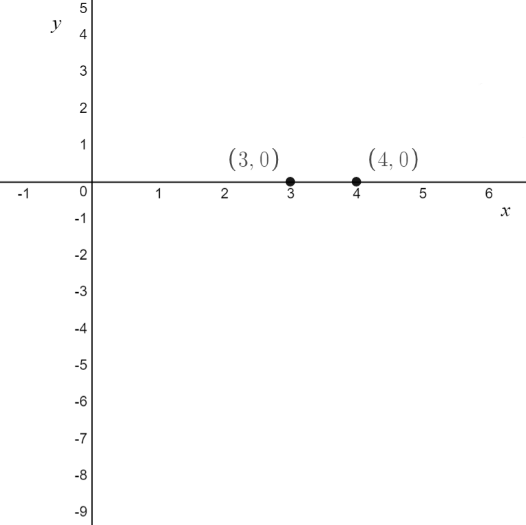
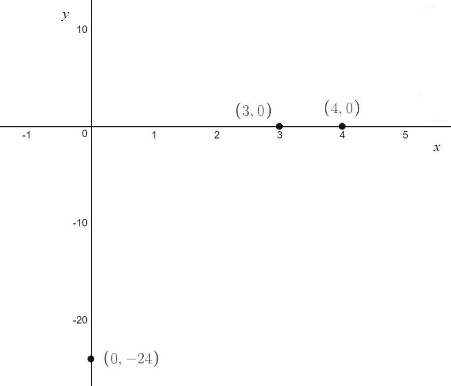
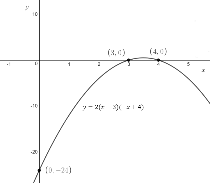
\[\text{Example 4.4: Sketch } f(x) = 2(x-3)(-x+4) \\ \text{ labelling any x-intercepts, y-intercepts and turning points}\]
\[
\text{1. Mark in the x-intercepts} \\
\begin{aligned}
x-3&=0\\
x&=3\\
-x+4&=0\\
4 &=x\\
\end{aligned}\\
\text{The x-intercepts have coordinates } (3,0) \text{ and } (4,0)
\]
\[
\text{ } \\
\text{5. The domain is not restricted. No changes need to be made}
\]
\[\text{Example 4.4: Sketch } f(x) = 2(x-3)(-x+4) \\ \text{ labelling any x-intercepts, y-intercepts and turning points}\]
\[
\text{1. Mark in the x-intercepts} \\
\begin{aligned}
x-3&=0\\
x&=3\\
-x+4&=0\\
4 &=x\\
\end{aligned}\\
\text{The x-intercepts have coordinates } (3,0) \text{ and } (4,0)
\]
 \[
\text{ } \\
\text{2. Find the y-intercept} \\
\begin{aligned}
x&= 0\\
y&= 2(0-3)(-0+4) \\
y&=2(-3)(4) \\
y&= -24 \\
\end{aligned}\\
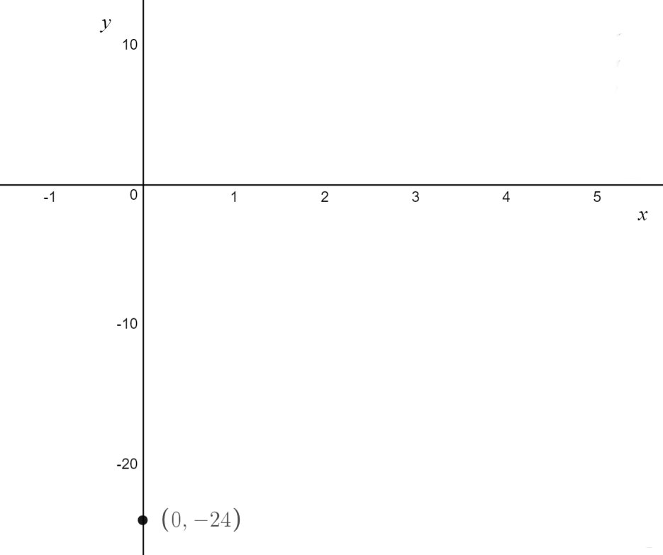
\text{There is a y-intercept at } (0,-24)
\]
\[
\text{ } \\
\text{2. Find the y-intercept} \\
\begin{aligned}
x&= 0\\
y&= 2(0-3)(-0+4) \\
y&=2(-3)(4) \\
y&= -24 \\
\end{aligned}\\
\text{There is a y-intercept at } (0,-24)
\]
 \[
\text{ } \\
\text{3. Connect the dots}
\]
\[
\text{ } \\
\text{3. Connect the dots}
\]
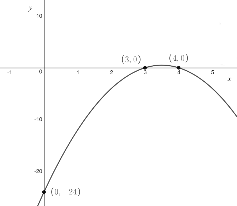 \[
\text{4. Label the equation}
\]
\[
\text{4. Label the equation}
\]
 \[
\text{ } \\
\text{5. The domain is not restricted. No changes need to be made}
\]
\[\text{Example 4.5: Sketch } f(x) = -2x^2+14x-24 \\ \text{ labelling any x-intercepts, y-intercepts and turning points}\]
\[
\text{1. Mark in the y-intercept} \\
\text{The y-intercepts has coordinates } (0,-24)
\]
\[
\text{ } \\
\text{5. The domain is not restricted. No changes need to be made}
\]
\[\text{Example 4.5: Sketch } f(x) = -2x^2+14x-24 \\ \text{ labelling any x-intercepts, y-intercepts and turning points}\]
\[
\text{1. Mark in the y-intercept} \\
\text{The y-intercepts has coordinates } (0,-24)
\]
 \[
\text{ } \\
\text{2. Find the x-intercepts} \\
\begin{aligned}
y&= 0\\
0&= -2x^2 +14x-24 \\
0&= -x^2+7x-12 \\
0&=x^2-7x+12 \\
0&= (x-4)(x-3) \\
\end{aligned}\\
x=3, 4\\
\text{There are x-intercepts at } (3,0) \text{ and } (4,0)
\]
\[
\text{ } \\
\text{2. Find the x-intercepts} \\
\begin{aligned}
y&= 0\\
0&= -2x^2 +14x-24 \\
0&= -x^2+7x-12 \\
0&=x^2-7x+12 \\
0&= (x-4)(x-3) \\
\end{aligned}\\
x=3, 4\\
\text{There are x-intercepts at } (3,0) \text{ and } (4,0)
\]
 \[
\text{ } \\
\text{3. Connect the dots}
\]
\[
\text{ } \\
\text{3. Connect the dots}
\]
 \[
\text{4. Label the equation}
\]
\[
\text{4. Label the equation}
\]
 \[
\text{ } \\
\text{5. The domain is not restricted. No changes need to be made}
\]
\[
\text{ } \\
\text{5. The domain is not restricted. No changes need to be made}
\]
The discriminant of a polynomial (in additive form) is: \[\triangle = b^2 - 4ac\] Note that this is what is inside the square root of the quadratic formula.
For the equation:
\[ax^2 + bx + c =0\]
The discriminant indicates how many solutions (x-intercepts) there will be.
If △ > 0, then there are two solutions
If △ = 0, then there is exactly one solutions
If △ < 0, then there are no (real) solutions
\[ \text{Example 4.6: Find the value(s) of }m \text{ for which } \\ f(x) = (4m+1)x^2-6mx+4\text{ is a perfect square (has one root). }\\ \text{ }\\ \text{A perfect square, has one solution. Thus, the discriminant will equal 0} \\ \begin{aligned} 0 &= (-6m)^2 - 4(4m+1)(4) \\ 0 &= 36m^2 -4(16m + 4) \\ 0 &= 36m^2 - 64m -16 \\ 0 &= 9m^2 -16m - 4 \\ 0 &= (9x+2)(x-2) \\ m &= 2, -\frac{2}{9} \\ \end{aligned}\\ \]
\[
\text{Example 4.7: Find the value(s) of }k\text{ for which }a(x) = b(x)\text{ will have exactly two solutions. }\\
\begin{aligned}
a(x) &= kx - 1\\
b(x) &= x^2 + 2x + 1\\
\text{ }\\
a(x) &= b(x) \\
kx - 1 &= x^2 + 2x + 1 \\
0 &= x^2 + 2x + 1 - kx + 1 \\
0 &= x^2 + (2-k)x \\
\text{ } \\
\end{aligned}\\
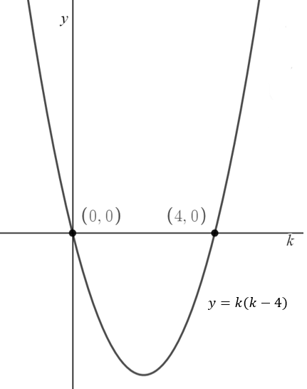
\text{The discriminant of that equation will be larger than zero as we are after exactly two solutions.} \\
\begin{aligned}
0 &< (2-k)^2-4 \cdot 1\\
0 &< 4 - 4k + k^2 - 4\\
0 &< k^2 -4k\\
0 &< k(k - 4) \\
\end{aligned}\\
k < 0 \text{ or } k >4 \text{ (from the graph } y=k(k-4)\text{)}
\]
The only way for two polynomials to ever be equal is if the coefficients of each corresponding term is equal. That is: \[a_{n}\cdot x^{n} + a_{(n-1)}\cdot x^{n-1} + … + a_{0}=b_{n}\cdot x^{n} + b_{(n-1)}\cdot x^{n-1} + … + b_{0}\] \[\implies a_{n} = b_{n} , \,a_{n-1}=b_{n-1},...,\,a_{0} = b_{0}\]
\[ \text{ }\\ \text{Example 4.8: Find the values of } a,b \text{ and } c \text{ if } ax^2+bx+c = 2(x-1)^2 + 1 \\ \begin{aligned} ax^2 + bx + c &= 2(x-1)^2 + 1 \\ ax^2 + bx + c &= 2(x^2 - 2x + 1) + 1 \\ ax^2 + bx + c &= 2x^2 - 4x + 3 \\ \end{aligned} \text{} \\ \text{So, } a = 2, b = -4 \text{ and } c = 3 \]
Division of polynomials is effectively the same as division with real numbers.
Below we show you an example of dividing \(3x^3-2x^2+3x-4\) by \(x^2-1\).
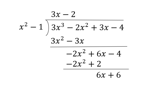
| 1 | Think - what expression can i multiply \(x^2-1\) so that the largest term will be \(3x^3\). That is \(3x\). |
| 2 | We want to multiply \(3x\) by \(x^2-1\) and write that under \(3x^3-2x^2+3x-4\). |
| 3 | Subtract \(3x^2-3\) from \(3x^3-2x^2+3x-4\) |
| 4 | Next we effectively repeat steps 1-3 except we think about getting the largest term of \(-2x^2\) - again the leading term. Here it is -2. |
| 5 | We want to multiply \(-2\) by \(x^2-1\) and write that under \(-2x^2+6x-4\) |
| 6 | Subtract \(-2x^2+2\) from \(-2x^2+6x-4\) |
| 7 | In the expression \(6x+6\), the highest degree (power) is 1. Thus, we cannot continue our division as we are dividing by an expression with degree 2 which is larger than 1. So, \(6x+6\) is the remainder |
The remainder theorem allows us to find the remainder of a polynomial when it is divided by a linear polynomial. \[\textrm{If a polynomial }P(x)\textrm{ is divided by }ax+b,\textrm{ then the remainder is equal to }P(-\frac{b}{a})\]
\[ \text{Example 4.9: Find the remainder of }f(x)\text{ when it is divided by g(x)}\\ \begin{aligned} f(x) &= x^3+x^2+x+1\\ g(x) &= 2x - 3\\ \end{aligned}\\ \] \[ \begin{aligned} \text{}f(-\frac{-3}{2}) &= f(\frac{3}{2})\\ &=(\frac{3}{2})^3 + (\frac{3}{2})^2 + (\frac{3}{2})+1\\ &=\frac{65}{8}\\ \end{aligned}\\ \therefore \text{The remainder is } \frac{65}{8} \]
The factor theorem effectively states the opposite of the remainder theorem. \[\text{If }P(-\frac{b}{a}) = 0,\text{ then }ax+b\text{ is a factor of }P(x)\]
\[ P(x) = a_{n}\cdot x^{n} + a_{n-1}\cdot x^{n-1} + … + a_{0}\\ \text{The rational root theorem states that if }ax+b\text{ is a factor of }P(x)\text{, that is }P(-\frac{b}{a}) = 0\\ \text{ and }a\text{ and }b\text{ have highest common factor of }1 \\ \text{, then }\pm b\text{ must be a factor of }a_{n}\text{ and }\pm a\text{ must be a factor of }a_{0}\\ \] Application of the rational root theorem is shown in the next section.
Factorising polynomials requires use of the rational root and factor theorems.
| 1 | Use the rational root theorem to find all the possible factors |
| 2 | Use the factor theorem to find a factor |
| 3 | Use long division to find the other factor(s) |
| 4 | Factorise the factor found in step 3 if possible |
\[ \text{Example 4.10: Factorise }P(x)=2x^3+x^2-6x-3\\ \text{ } \\ \text{The coefficient of the leading term here is } 2, \text{ factors of } 2 \text{ are }: \, 1, 2\\ \text{The constant term here is } -3, \, \text{ factors of } 3 \text{ are }: \, 1, 3 \\ \]
So, using the rational root theorem, we want to get all of the factors of the constant term and divide them by the factors of the coefficient of the leading term. Having got that list, we want to add a plus or minus sign in front of each value to remind us to check those values too. We get the following values:
\[ \pm \frac{3}{1} , \pm \frac{3}{2}, \pm \frac{1}{2}, \pm \frac{1}{1} \\ \text{ }\\ \text{Substituting each of those values into } P(x) \text{ the first one which yields } 0 \text{ is:}\\ P(-\frac{1}{2}) = 0 \\ \text{So, } 2x+1 \text{ is a factor of } P(x) \\ \text{ } \\ \text{Using long division, } \frac{P(x)}{(2x+1)} = x^2 -3 \\ \begin{aligned} \text{So, } P(x) &= (2x+1)(x^2-3) \\ &= (2x+1)(x+\sqrt{3})(x-\sqrt{3}) \\ \end{aligned} \]\[x^3-a^3 = (x-a)(x^2+ax+a^2)\\ x^3+a^3 = (x+a)(x^2-ax+a^2)\]
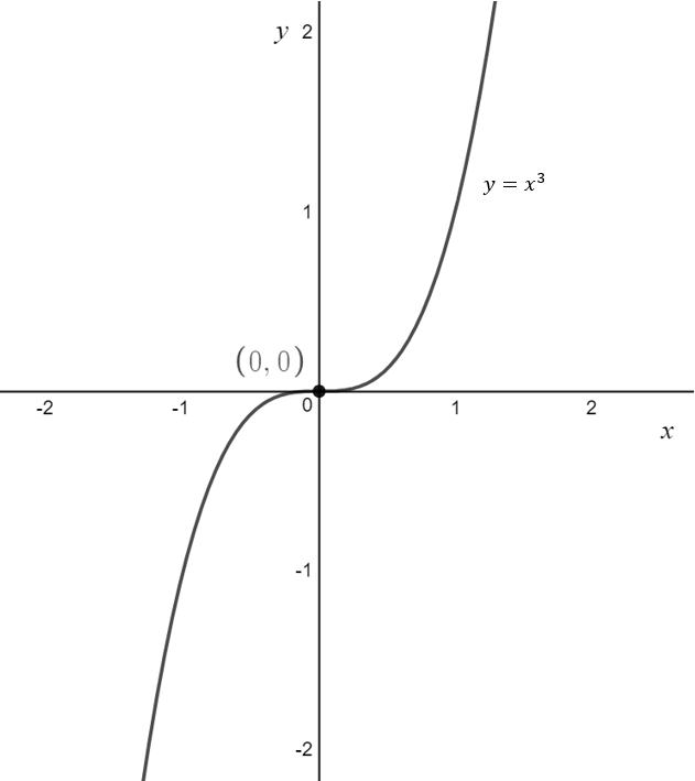
The basic shape of a cubic is shown below
In general, unless told not to, all graphs must provide the coordinates or equations of any: x-intercepts, y-intercepts and asymptotes. There are three different ways to graph quadratics.
Method 1 - Use when provided equation in stationary point of inflection form \[y = a(x-h)^3 + k\]
| 1 | Mark out the coordinate of the stationary point of inflection at (h,k) |
| 2 | Substitute x = 0 into the equation and solve for y to find the y-intercept |
| 3 | Substitute y = 0 into the equation and solve for x to find the x-intercept(s) (you will need to expand the quadratic expression) |
| 4 | Determine roughly where your graph starts. If a > 0 then your graph will commence in the bottom left corner and move towards the top right corner. If a < 0 then your graph will commence in the top left corner and move bottom right corner. |
| 5 | Connect the dots appropriately |
| 6 | Adjust the graph according to the domain, finding the coordinates of the endpoints if required. Label with the equation. |
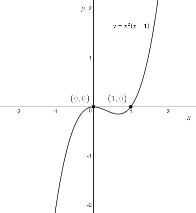
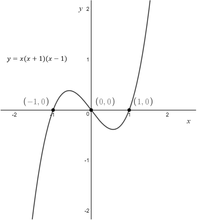
Method 2 - Use when provided equation in product (intercept) form \[y = a(x-b)(x-c)(x-d)\]
| 1 | Mark out the coordinates of the x-intercepts at (b,0), (c,0) and (d,0). |
| 2 | Substitute x = 0 into the equation and solve for y to find the y-intercept |
| 3 | Determine where your graph starts. If a > 0 then your graph will commence in the bottom left corner and move towards the top right corner. If a < 0 then your graph will commence in the top left corner and move bottom right corner. For every negative coefficient in front of a x < 0 you will need to switch to the other option. View examples for more details. |
| 4 | Connect the dots appropriately. If a factor is repeated, the graph will produce a turning point at the x-intercept. |
| 5 | Adjust the graph according to the domain, finding the coordinates of the endpoints if required. Label with the equation. |
Method 3 - Use when provided equation in additive (expanded) form \[y = ax^3+bx^2+cx+d\]
| 1 | Mark out the coordinates of the y-intercepts at (0,d) |
| 2 | Substitute y = 0 into the equation and solve for x to find the x-intercept(s) (you will need to expand the quadratic expression) |
| 3 | Determine where your graph starts. If a > 0 then your graph will commence in the bottom left corner and move towards the top right corner. If a < 0 then your graph will commence in the top left corner and move bottom right corner. |
| 4 | Connect the dots appropriately |
| 5 | Adjust the graph according to the domain, finding the coordinates of the endpoints if required. Label with the equation. |
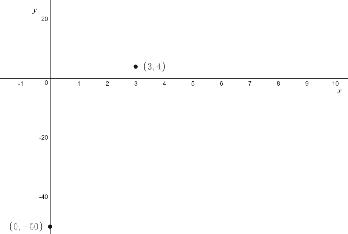
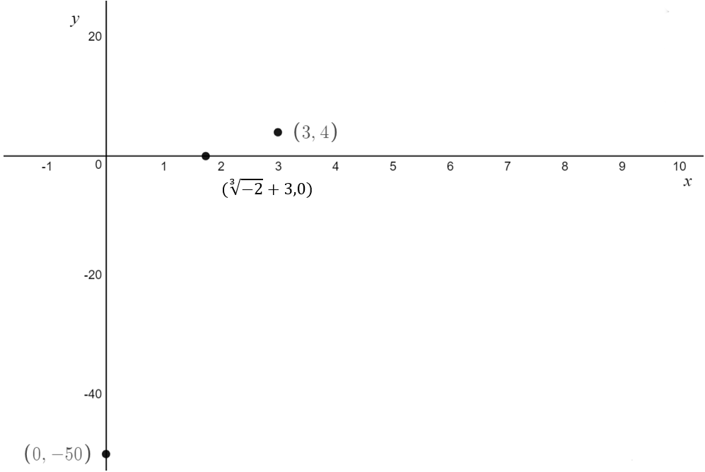
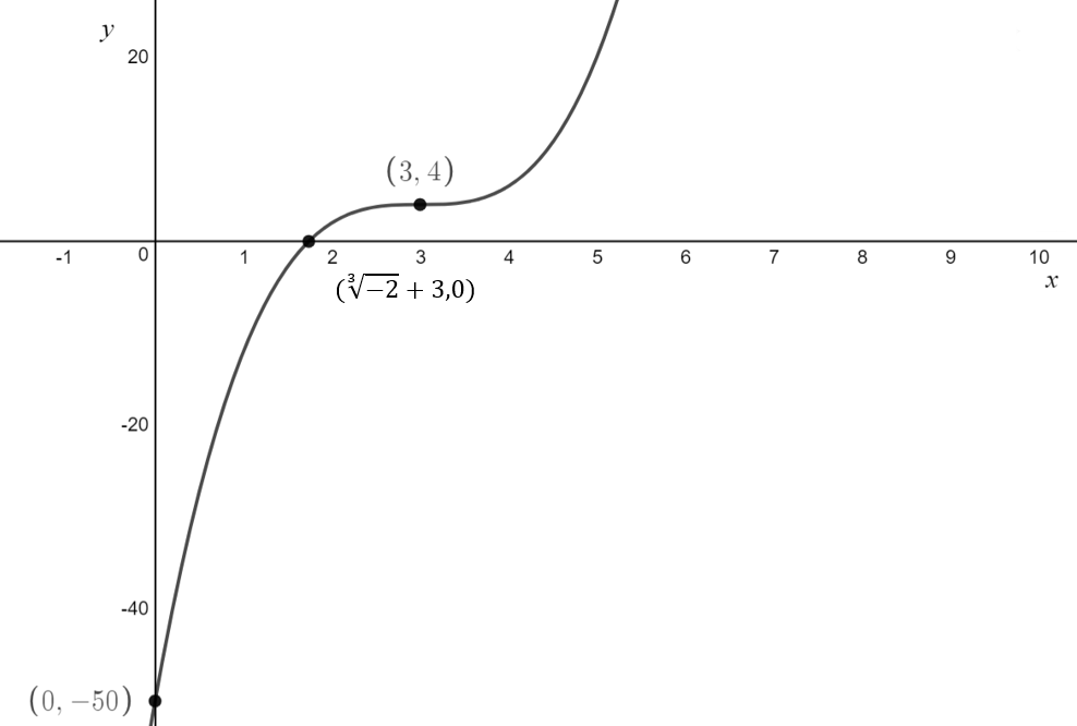
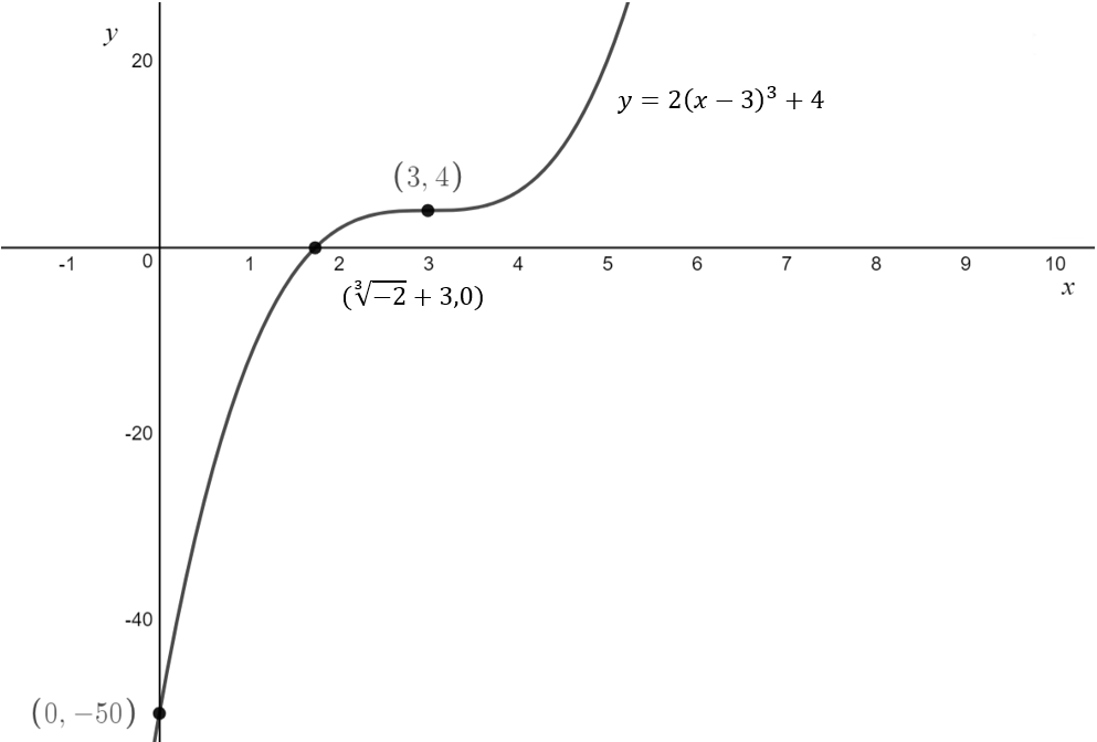
\[\text{Q. Sketch} f(x) = 2(x-3)^3+4 \text{ labelling any x-intercepts, y-intercepts and turning points}\]
\[
\text{1. Mark in the stationary point of inflection} \\
\text{The stationary point of inflection has coordinates } (3,4)
\]
 \[
\text{ } \\
\text{2. Find the y-intercept} \\
\begin{aligned}
x&= 0\\
y&= 2(0-3)^3+4 \\
y&= 2 \cdot (-27) + 4 \\
y &= -54 + 4\\
y&= -50\\
\end{aligned}\\
\text{There is a y-intercept at } (0,-50)
\]
\[
\text{ } \\
\text{2. Find the y-intercept} \\
\begin{aligned}
x&= 0\\
y&= 2(0-3)^3+4 \\
y&= 2 \cdot (-27) + 4 \\
y &= -54 + 4\\
y&= -50\\
\end{aligned}\\
\text{There is a y-intercept at } (0,-50)
\]
 \[
\text{ } \\
\text{3. Find the x-intercepts} \\
\begin{aligned}
y&=0\\
0&=2(x-3)^3+4\\
-\frac{4}{2} &= (x-3)^3\\
\sqrt[3]{-2} &= x-3\\
\sqrt[3]{-2} + 3 &= x\\
\end{aligned}\\
\text{This is a x-intercept at } (\sqrt[3]{-2} + 3, 0)\\
\]
\[
\text{ } \\
\text{3. Find the x-intercepts} \\
\begin{aligned}
y&=0\\
0&=2(x-3)^3+4\\
-\frac{4}{2} &= (x-3)^3\\
\sqrt[3]{-2} &= x-3\\
\sqrt[3]{-2} + 3 &= x\\
\end{aligned}\\
\text{This is a x-intercept at } (\sqrt[3]{-2} + 3, 0)\\
\]
 \[
\text{ } \\
\text{4. Connect the dots}
\]
\[
\text{ } \\
\text{4. Connect the dots}
\]
 \[
\text{4. Label the equation}
\]
\[
\text{4. Label the equation}
\]
 \[
\text{ } \\
\text{5. The domain is not restricted. No changes need to be made}
\]
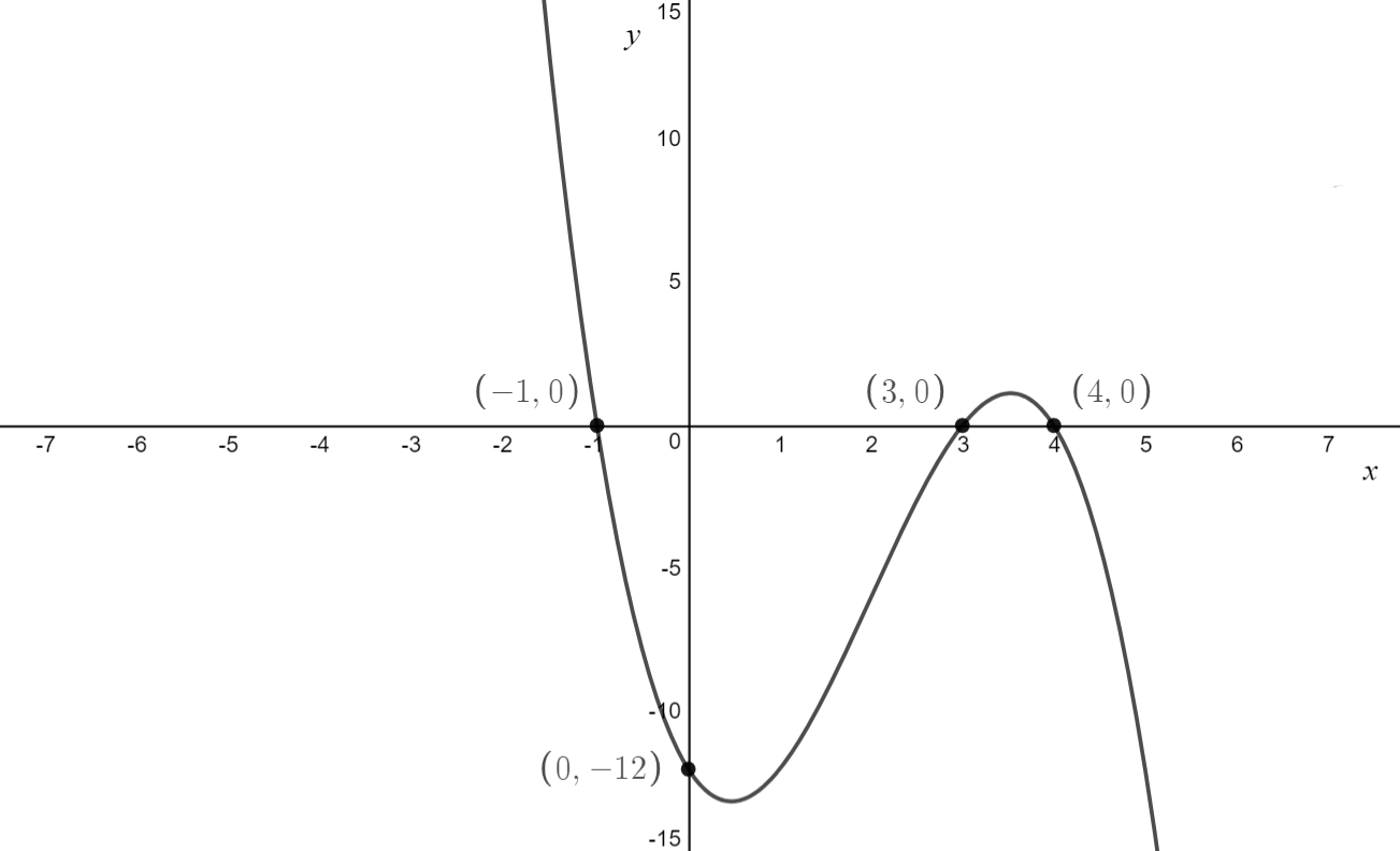
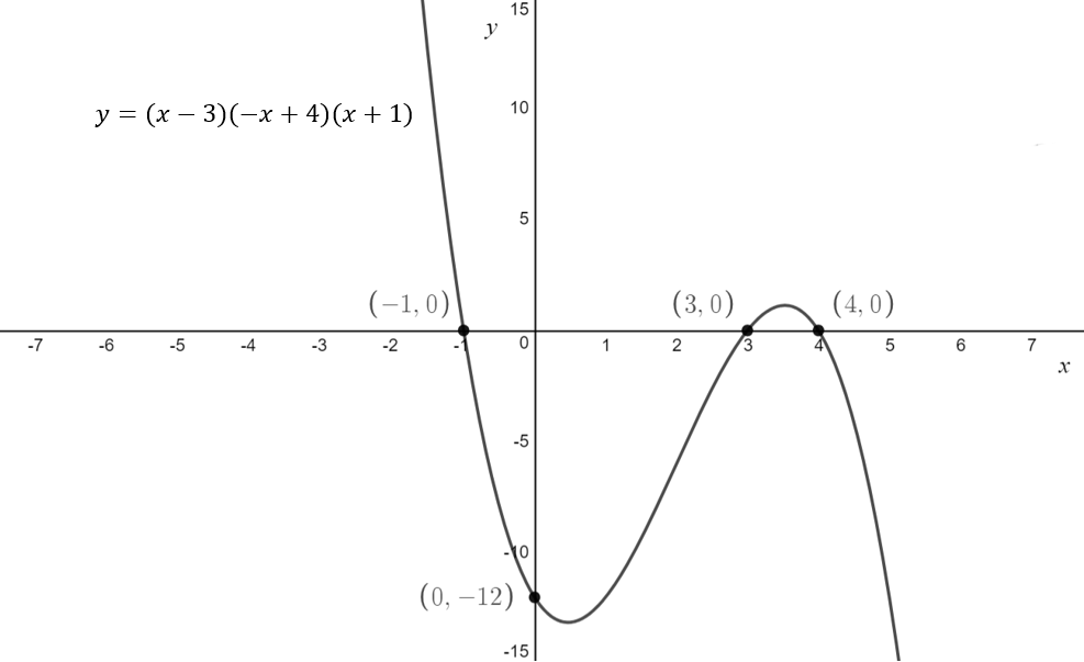
\[\text{Q. Sketch} f(x) = 2(x-3)(-x+4)(x+1) \\ \text{ labelling any x-intercepts, y-intercepts and turning points}\]
\[
\text{1. Mark in the x-intercepts} \\
\begin{aligned}
x-3&=0\\
x&=3\\
-x+4&=0\\
4 &=x\\
x+1&=0\\
x&=-1\\
\end{aligned}\\
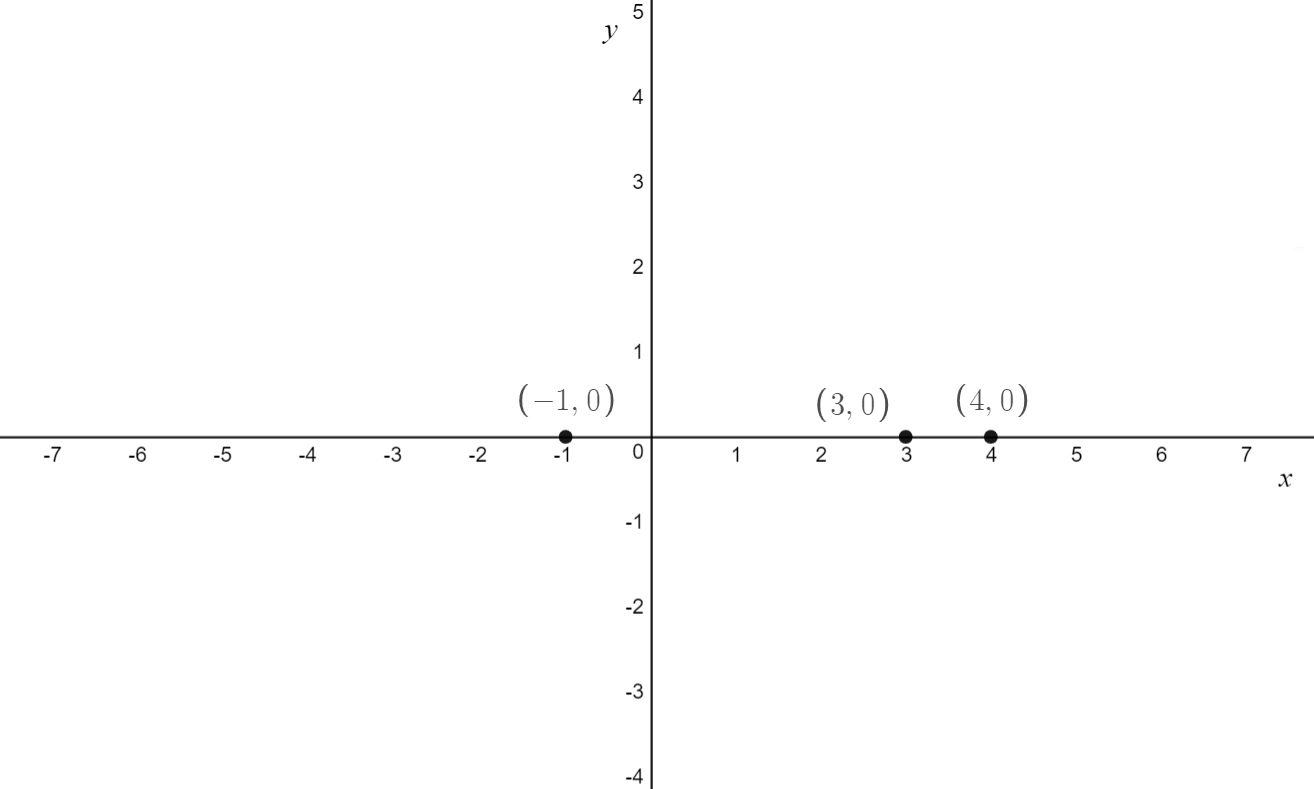
\text{The x-intercepts have coordinates } (-1,0), \, (3,0) \text{ and } (4,0)\\
\]
\[
\text{ } \\
\text{5. The domain is not restricted. No changes need to be made}
\]
\[\text{Q. Sketch} f(x) = 2(x-3)(-x+4)(x+1) \\ \text{ labelling any x-intercepts, y-intercepts and turning points}\]
\[
\text{1. Mark in the x-intercepts} \\
\begin{aligned}
x-3&=0\\
x&=3\\
-x+4&=0\\
4 &=x\\
x+1&=0\\
x&=-1\\
\end{aligned}\\
\text{The x-intercepts have coordinates } (-1,0), \, (3,0) \text{ and } (4,0)\\
\]
 \[
\text{ } \\
\text{2. Find the y-intercept} \\
\begin{aligned}
x&= 0\\
y&=(0-3)(-0+4)(0+1) \\
y&=(-3)(4)(1) \\
y&= -12 \\
\end{aligned}\\
\text{There is a y-intercept at } (0,-12)
\]
\[
\text{ } \\
\text{2. Find the y-intercept} \\
\begin{aligned}
x&= 0\\
y&=(0-3)(-0+4)(0+1) \\
y&=(-3)(4)(1) \\
y&= -12 \\
\end{aligned}\\
\text{There is a y-intercept at } (0,-12)
\]
 \[
\text{ } \\
\text{3. Connect the dots}
\]
\[
\text{ } \\
\text{3. Connect the dots}
\]
 \[
\text{4. Label the equation}
\]
\[
\text{4. Label the equation}
\]
 \[
\text{ } \\
\text{5. The domain is not restricted. No changes need to be made}
\]
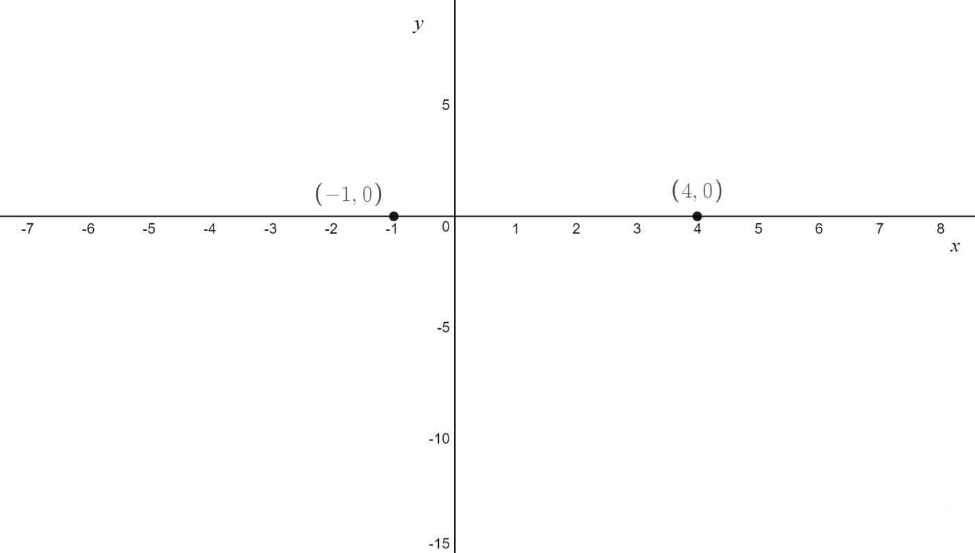
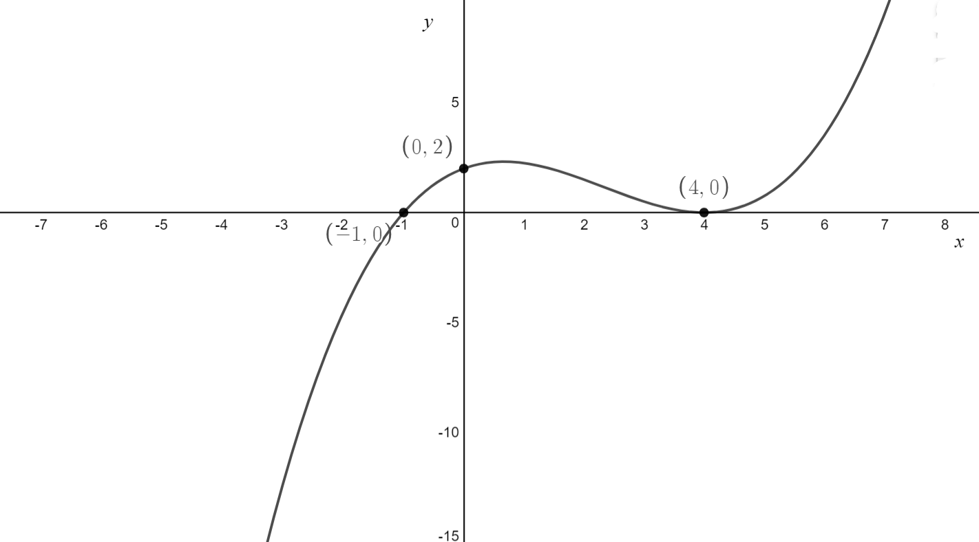
\[\text{Q. Sketch} f(x) = 2(x-3)(-x+4)^2 \text{ labelling any x-intercepts, y-intercepts and turning points}\]
\[
\text{1. Mark in the x-intercepts} \\
\begin{aligned}
x-3&=0\\
x&=3\\
x+1&=0\\
x &=1\\
\end{aligned}\\
\text{The x-intercepts have coordinates } (-1,0) \text{ and } (4,0)\\
\]
\[
\text{ } \\
\text{5. The domain is not restricted. No changes need to be made}
\]
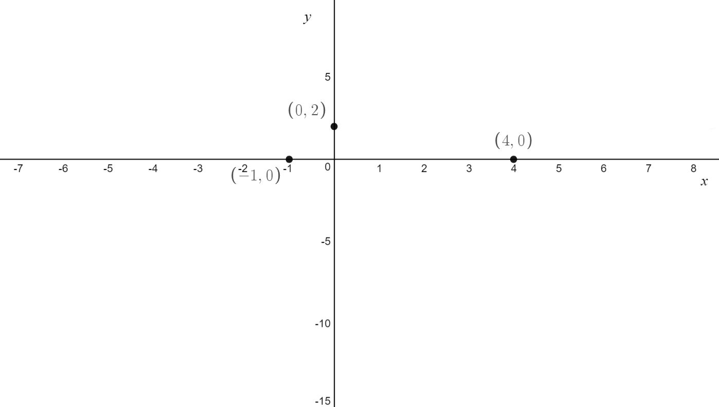
\[\text{Q. Sketch} f(x) = 2(x-3)(-x+4)^2 \text{ labelling any x-intercepts, y-intercepts and turning points}\]
\[
\text{1. Mark in the x-intercepts} \\
\begin{aligned}
x-3&=0\\
x&=3\\
x+1&=0\\
x &=1\\
\end{aligned}\\
\text{The x-intercepts have coordinates } (-1,0) \text{ and } (4,0)\\
\]
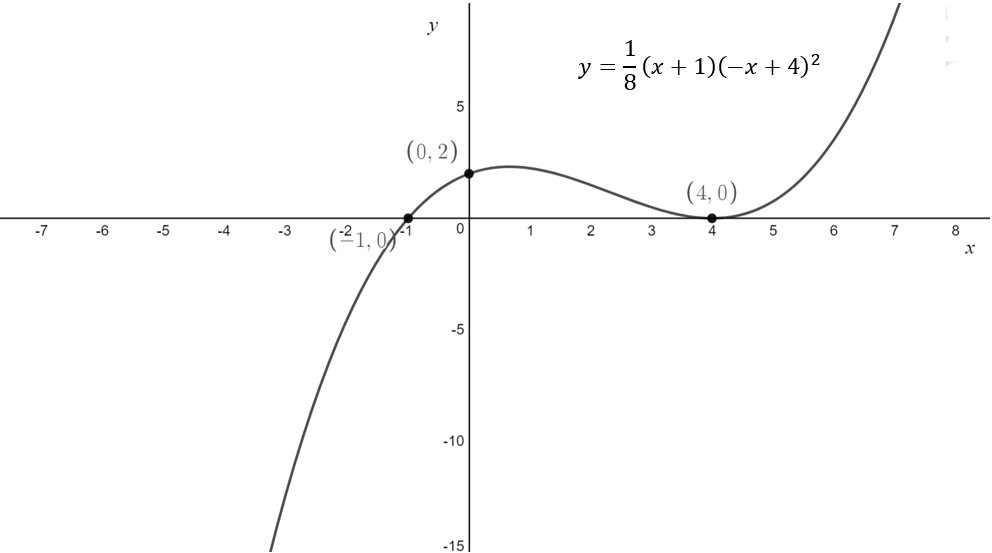
 \[
\text{ } \\
\text{2. Find the y-intercept} \\
\begin{aligned}
x&= 0\\
y&=\frac{1}{8}(0+4)^2(0+1)\\
y&=\frac{1}{8}(4)^2(1) \\
y&= 2 \\
\end{aligned}\\
\text{There is a y-intercept at } (0,2)
\]
\[
\text{ } \\
\text{2. Find the y-intercept} \\
\begin{aligned}
x&= 0\\
y&=\frac{1}{8}(0+4)^2(0+1)\\
y&=\frac{1}{8}(4)^2(1) \\
y&= 2 \\
\end{aligned}\\
\text{There is a y-intercept at } (0,2)
\]
 \[
\text{ } \\
\text{3. Connect the dots}
\]
\[
\text{ } \\
\text{3. Connect the dots}
\]
 \[
\text{4. Label the equation}
\]
\[
\text{4. Label the equation}
\]
 \[
\text{ } \\
\text{5. The domain is not restricted. No changes need to be made}
\]
\[
\text{ } \\
\text{5. The domain is not restricted. No changes need to be made}
\]
Polynomials of a higher degree than 3 are very rarely examined.
It is important to remember that the factor, remainder and rational root theorems which we learnt for cubics apply for all polynomials. Thus, if ever asked to solve a quartic, quintic ...etc. simply apply the same techniques.
If asked to graph a quartic, quintic… etc. we recommend first factorising the expression into product (intercept) form. From there, the shape of the curve at an x-intercept is determined by the power to which the factor is raised. If the factor is raised to an even power, it will have a turning point like intercept. If the factor is raised to an odd (excluding 1) power then it will have a stationary point of inflection like intercept. Any factor which is repeated exactly once, will have the graph cut through that point on the x-axis. We also know that the y-intercept will be the constant value of the polynomial function.
The general shape of a polynomial with an even degree (highest power) is found the same way as a quadratic. If the leading term has a positive coefficient, it will open upwards. If it has a negative coefficient it will open downwards.
The general shape of a polynomial with an odd degree (highest power) is found the same way as a cubic. If the leading term has a positive coefficient, the graph will move from the bottom left to top right. If it has a negative coefficient it will move from the top left to the bottom right.
From here roughly connect up all the intercepts we know taking into account the general shape of the graph. This can be done more precisely with calculus, we will discuss this more in later chapters.
Remember. The graph of any polynomial has exactly one y-intercept and at most n x-intercepts, where n is the degree (highest power) of the polynomial.
There are three different types of ‘determine the rule’ questions for polynomials.
Random points.
For any given polynomial, we need n+1 points to find its equation, where n is the degree of the polynomial. To do this, we simply substitute the x and y values into the additive form of the polynomial equation and solve the system of equations provided.
\[y = a_{n} \cdot x^{n} + a_{n-1} \cdot x^{n-1} + … + a_{0}\]
x-intercepts and one random point
If provided with all the x-intercepts we can use the product (intercept) form for polynomials. If the graph cuts through the x-axis, the factor will appear once in the equation. If there the graph forms a turning point at the x-axis, the factor will appear an even number of times (generally two when dealing with quadratics and cubics). If the graph forms a stationary point of inflection at the x-axis, the factor will appear an odd number of times (generally three).
To find the value of A simply substitute the x and y-coordinate of the additional point into the equation and solve for A.
\[y = A(x-a_{0})(x-a_{1})(x-a_{2})...(x-a_{n})\]
The turning point or stationary point of inflection and a random point
Using the turning point or stationary point of inflection form of the quadratic or cubic equations will allow us to efficiently determine the equation here.
\[\text{For a quadratic: } y = A(x-h)^2+k\]
\[\text{For a cubic: } y = A(x-h)^3 +k\]
\[\text{In general: } y = A(x-h)^n + k \text{ (Very unlikely to ever be used)}\]
In all cases, h is the x-coordinate of the turning point/ stationary point of inflection and k is the y-coordinate of the turning point/stationary point of inflection.
To find the value of A simply substitute the x and y-coordinate of the additional point into the equation and solve for A.
There are three methods for solving a pair simultaneous equations.
| 1 | Elimination - attempting to manipulate the equations provided and then adding/subtracting/multiply/dividing them to get rid of one unknown. This can often be quite difficult unless dealing with a pair of linear equations. |
| 2 | Graphically - Graphing the two equations and looking at the intersection point. This is not accurate. |
| 3 | Substitution - Re-arranging one of the equations making one of the unknowns the subject and then substituting that into the other equation. Often the best method when not dealing with a pair of linear equations. |
\[ \text{Example 4.11: Find the coordinates of the intersection points between the graphs with equations}\\ (x-2)^2+(y+3)^2=4 \text{ and } x-2y=6 \\ \text{ }\\ (x-2)^2+(y+3)^2=4 ... \boxed{1} \\ x - 2y = 6 \\ x=2y+6...\boxed{2}\\ \text{ }\\ \begin{aligned} \boxed{2}& \rightarrow \boxed{1}\\ \text{ }\\ \quad(2y+6-2)^2+(y+3)^2&=4\\ 4y^2+16y+16+y^2+6y+9&=4\\ 5y^2+22y+21&=0\\ 5y^2+15y+7y+21&=0\\ (5y+7)(y+3)&=0\\ y&=-3,\,-\frac{7}{5}\\ \end{aligned}\\ \text{Substitute the values of }y\text{ into }\boxed{2}\text{ to solve for x}\\ \therefore \text{Intersection points are at } (0,-3),\,(\frac{16}{5},-\frac{7}{5}) \]