VCEMethods


Differentiation
In differentiation we are concerned with rates of change, that is, how fast things are changing. For example: How fast is a car moving? How much is a car speeding up by? How is the slope of the land changing?
The derivative of a function tells us the slope (gradient) of the function at each specific x value.
The derivative can be represented in many ways. The derivative of \[y = f(x)\] can be represented as:
\[y' = f'(x) = \frac{dy}{dx}\]
Differentiation by first principles involves finding the gradient (average rate of change - discussed further below) of a function with respect to x over an interval
[x, x + h] and considering what happens as h approaches zero.
\[\frac{dy}{dx} = \lim_{h \to 0} \frac{f(x+h) - f(x)}{x+h-x}\]
With first principles questions you should first fully expand the expression on the right hand side, then simplify that expression before substituting h = 0 into the expression. You cannot skip the expansion and simplification steps as substituting h = 0 straight away will result in an undefined fraction (denominator cannot equal to zero). More information on working with limits is presented in the limits section of this page below. Do not find derivatives using first principles unless the question explicitly asks for you to do it this way.
\[ \text{ }\\ \text{Example 7.1: Using first principles, find the derivative of the function } f(x) = x^2-2x+3\\ \begin{aligned} f’(x) &= \lim_{h \to 0} \frac{f(x+h) - f(x)}{x+h-x}\\ f’(x) &= \lim_{h \to 0} \frac{(x+h)^2-2(x+h) + 3 - (x^2-2x+3)}{h}\\ f’(x) &= \lim_{h \to 0} \frac{x^2 + 2xh + h^2 -2x - 2h + 3 - x^2 + 2x -3}{h}\\ f’(x) &= \lim_{h \to 0} \frac{h^2 + 2xh - 2h}{h}\\ f’(x) &= \lim_{h \to 0} h + 2x - 2\\ f’(x) &= 2x - 2\\ \end{aligned}\\ \]
| \[f(x)=c \rightarrow f’(x)=0\, , c \in \mathbb{R}\] | \[f(x)=k \cdot g(x) \rightarrow f’(x)=k \cdot g’(x)\, , k \in \mathbb{R}\] |
| \[f(x)=g(x) + h(x) \rightarrow f’(x)= g’(x) + h’(x)\] | \[f(x)=g(x) - h(x) \rightarrow f’(x)= g’(x) - h’(x)\] |
| \[(x^n)’ = n \cdot x^{n-1}\] | \[((ax+b)^n)’ = a \cdot n(ax+b)^{n-1}\] |
| \[(\log_{e}{x})’ = \frac{1}{x}\] | \[(\sin(ax))’ = a \cdot \cos(ax)\] |
| \[(\cos(ax))’ = -a \cdot \sin(ax)\] | \[(\tan(ax))’ = \frac{a}{\cos^2(ax)} = a \cdot \sec^2(ax)\] |
A function is strictly increasing on an interval [a,b] if f(a) < f(b).
A function is strictly decreasing on an interval [a,b] if f(a) > f(b).
A function is increasing on an interval [a,b] if f’(x) > 0 for the entire interval.
A function is decreasing on an interval [a,b] if f’(x) <0 for the entire interval.
The chain rule is used to differentiate composite functions, that is when there is a function within a function. We use the chain rule when we know how to differentiate the two individual functions, but not when they have been put together. Revise the “Composite functions” section in chapter one if you are unable to recognise composite functions.
\[ y=f(g(x))\\ \frac{dy}{dx} = \frac{dy}{du} \cdot \frac{du}{dx} \text{, where } u = g(x)\\ \text{ }\\ \text{ }\\ \text{Example 7.2: Differentiate each of the following: }\\ \text{ }\\ \text{Q. } y = (x^2 + 3)^{12}\\ \text{The “inner” function } (g(x)) \text{ is } x^2 + 3\\ \begin{aligned} \text{Let } u &= x^2 + 3\\ \text{So, } y &= u^{12}\\ \frac{du}{dx} &= 2x\\ \frac{dy}{du} &= 12u^{11}\\ \frac{dy}{dx} &= \frac{dy}{du} \cdot \frac{du}{dx}\\ &= 12u^{11} \cdot 2x\\ (&\text{Substituting } u=x^2 + 3)\\ &= 12(x^2 + 3)^{11} \cdot 2x\\ &= 24x(x^2 + 3)^{11}\\ \end{aligned}\\ \text{ }\\ \text{Always remember to substitute } x \text{ back into the equation, never leave} \\ \text{ unknowns which you have created in your final answer.}\\ \text{ }\\ \text{Example 7.3: } y =\sin(\log_{e}{x})\\ \text{The “inner” function} (g(x)) \text{is} \log_{e}{x}\\ \begin{aligned} \text{Let } u &= \log_{e}{x}\\ \text{And, } y &= \sin(u)\\ \frac{du}{dx} &= \frac{1}{x}\\ \frac{dy}{du} &= \cos(u)\\ \frac{dy}{dx} &= \frac{dy}{du} \cdot \frac{du}{dx}\\ &= \cos(u) \cdot \frac{1}{x}\\ (&\text{Substituting } u = \log_{e}{x})\\ &= \cos(\log_{e}{x}) \cdot \frac{1}{x}\\ &= \frac{\cos(\log_{e}{x})}{x}\\ \end{aligned}\\ \]
Use the product rule when you want to know the derivative of a function which is the product of two functions.
Use the quotient rule when you want to know the derivative of a function which a function divided by another function.
\[(f(x) \cdot g(x))’ = f’(x) \cdot g(x) + f(x) \cdot g’(x) \]
\[(\frac{f(x)}{g(x)})’ = \frac{f’(x) \cdot g(x) - f(x) \cdot g’(x)}{[g(x)]^2}\]
This topic is not so important in methods and can be hard to understand. However, there is only really one core concept to understand.
With limits, we are concerned with the value our graph is approaching (not to be confused with equal) at a given x-value from the left hand side and right hand side. If the value of y is approaching a non finite number (infinity, or different values), then the limit is undefined. We have provided examples below to help you understand this.
\[ \lim_{x \to a} f(x) = b \text{ As the } x \text{ value approaches } a, \text{ the graph approaches } b \text{ from the left and right hand side}. \\ \lim_{x \to a^-} f(x) = b \text{ As the } x \text{ value approaches } a, \text{ the graph approaches } b \text{ from the left hand side}. \\ \lim_{x \to a^+} f(x) = b \text{ As the } x \text{ value approaches } a, \text{ the graph approaches } b \text{ from the right hand side}. \]
\[
\text{Looking at the graph of } y = x^2 \text{ , we can see that at } x= 0 \text{ the } y \text{ value approaches } 0.\\ \text{ Mathematically: } \\
\lim_{x \to 0} x^2 = 0
\]

\[
\text{Looking at the graph of } y = \frac{1}{x^2} \text{ , we can see that at } x= 0 \text{ the } y \text{ value approaches } \infty.\\ \text{Thus, the limit is undefined.} \text{ Mathematically: } \\
\lim_{x \to 0} \frac{1}{x^2} \text{ is undefined}
\]

Looking at the two linear graphs , we can see that at \(x= 0\) the \(y\) value approaches \(-\frac{1}{2}\) from the left hand side for the graph at the bottom (even though the point is undefined) and \(\frac{1}{2}\) for the graph at the top from the right hand side. Thus, the limit is undefined. However, we can describe how the two functions approach their respective values. Mathematically:
\[
f(x) =
\begin{cases}
-0.5 & x < 0 \\
0.5 & x > 0\\
\end{cases}\\
\lim_{x \to 0^-} f(x) = -0.5 \\
\lim_{x \to 0^+} f(x) = 0.5 \\
\lim_{x \to 0} f(x) \text{ is undefined}
\]

Looking at the graph of \(y =x\) . There is a point of discontinuity at \(x = 0\) and the y value is 1. But, at \(x= 0\) the \(y\) value clearly approaches towards \(0\) from both left and right hand sides. Thus, the limit is defined and equal to \(0\). Mathematically:
\[
f(x) =
\begin{cases}
x & x < 0 \\
1 & x = 0\\
x & x > 0 \\
\end{cases}\\
\lim_{x \to 0} f(x) = 0
\]

Almost always in methods, if the limit is defined, it is true that: \[\lim_{x \to a} f(x) = f(a)\] However, as shown in the final example, this is not always the case. Thus, it is best to consider the graphs of the functions presented and see what value(s) x is approaching.
A function is considered to be continuous if you can graph the whole thing without taking your pen off the page and moving it to a different position.
A function is considered to be discontinuous at a point when you have to take your pen off the page and move it to continue the graph.
In a more mathematical statement, a function is continuous at the point where x = a if : \[f(a) = \lim_{x \to a^+}f(x) = \lim_{x \to a^-}f(x)\] That is, the function is defined at the point a and approaches that value from the left and right.
A function is only differentiable at a point (a, f(a)) if the function is both continuous (discussed above) and smooth (the gradient approaches the same value from the left and right) at that point.
A function is considered to be smooth at the point x = a if:
\[\lim_{h \to 2^+}\frac{f(x+h)-f(x)}{h} = \lim_{h \to 2^-}\frac{f(x+h)-f(x)}{h}\]
An example of a point which is not smooth is that at (0,0)

Just like addition of ordinates, you are not expected to produce a perfect graph. There are a few key points which we detail below which you must get correct. For all the other points in the graph, something of the correct shape roughly in the right spot will be awarded full marks.
| 1 | For Any horizontal line, the graph of the derivative will have equation y = 0. That is it will be a horizontal line which lies on the x-axis |
| 2 | For any linear equations, calculate the gradient exactly (if not possible, approximate). The graph of the derivative will have equation y = gradient. That is a horizontal line with a y-intercept at the value of the gradient. |
| 3 | Any point which looks like a stationary point. The derivative graph will have an x-intercept with the corresponding x-value. Mark in these points. |
| 4 | Approximate the gradient of any other sections of the graph which are presented and draw them in making sure that you go through the x-intercepts which you have already marked in if any. |
| 5 | Any endpoints or points of discontinuity, whether the points are inclusive or exclusive on the original graph, will be undefined (open circle) on the graph of the derivative. |
| 6 | Any sharp points on the original graph, the corresponding x-value on the graph of the derivative will have an undefined (open circle) point. |
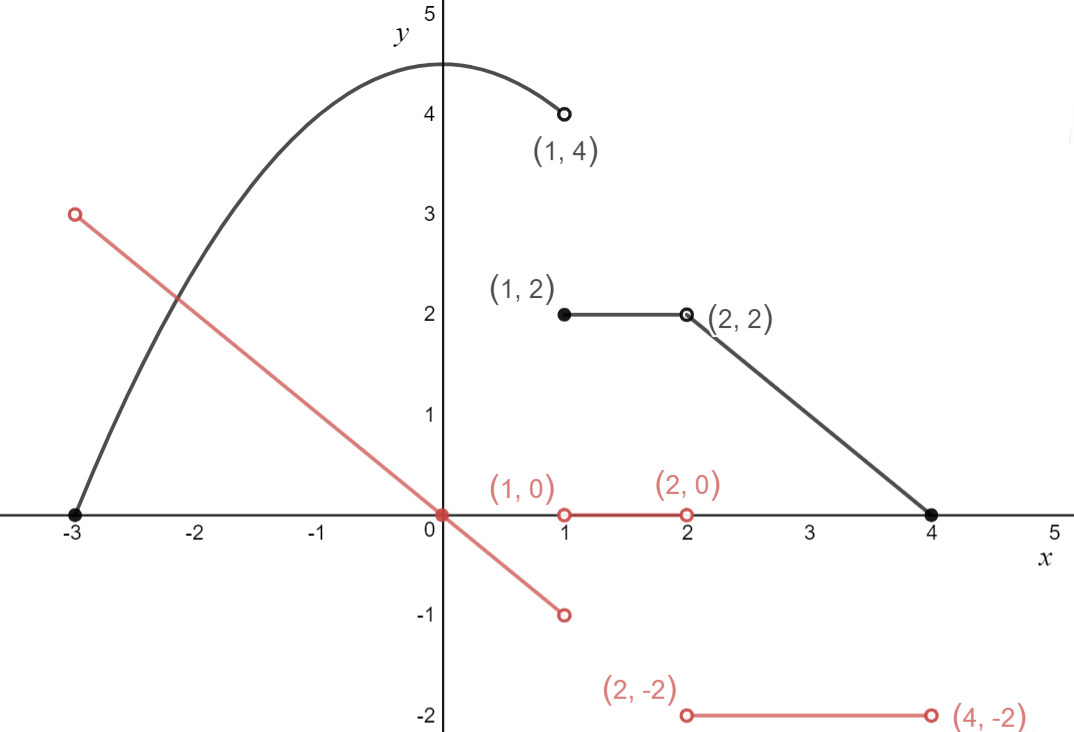
\[
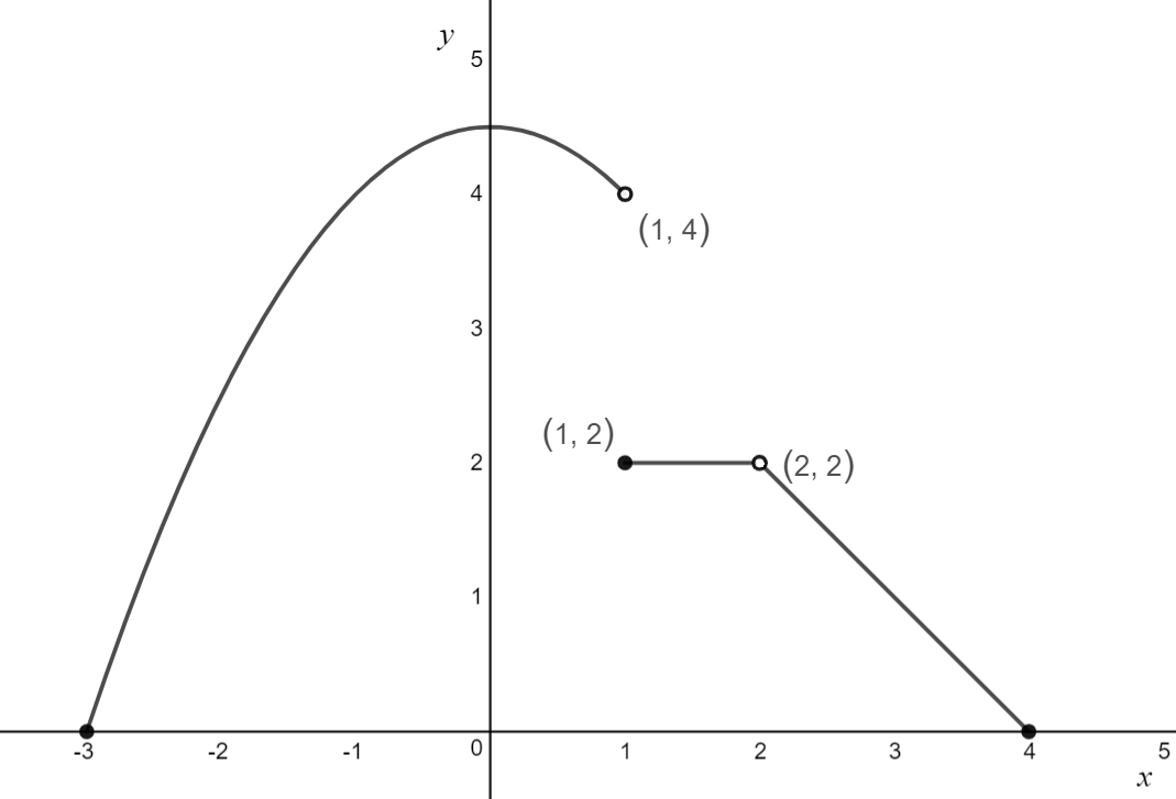
\text{Example 7.4: A piecewise function is shown below.}\\ \text{ Sketch the derivative function on the same set of axis.}\\
\text{ }
\]
\[
\text{ }\\
\text{We have sketched the derivative graph in red.} \\
\text{1. Deal with any horizontal lines} \\
\]
\[
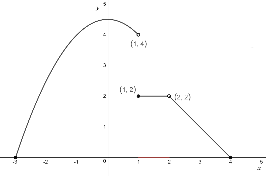
\text{ }\\
\text{2. Deal with any linear lines}\\
\begin{aligned}
m &= \frac{2-0}{2-4}\\
m &= -2 \\
\end{aligned}\\
\]

\[
\text{ }\\
\text{3. Dot in stationary points}\\
\]

\[
\text{ }\\
\text{4. Approximate rest of the graph}\\
\]
\[
\text{ }\\
\text{5. Deal with endpoints and sharp points}\\
\]
Finding the equation of the tangent line to the function y = f(x) at x = a
| 1 | Find f ’(x) |
| 2 | Evaluate f ’(a) |
| 3 | Evaluate f(a) |
| 4 | Equation of tangent: y - f(a) = f ’(a) ∙ (x-a) |
| 5 | Rearrange for y: y = f ’(a) ∙ (x-a) + f(a) |
Finding the equation of the normal line to the function y = f(x) at x = a
| 1 | Find f ’(x) |
| 2 | Evaluate f ’(a) |
| 3 | Find m, the gradient of the normal - m ∙ f ’(a) = -1 [Only step which is different to finding tangent line] |
| 4 | Evaluate f(a) |
| 5 | Equation of tangent: y - f(a) = m ∙ (x-a) |
| 6 | Rearrange for y: y = m ∙ (x-a) + f(a) |
\[ \text{Example 7.5: Find the equation of the tangent and normal lines to the function }\\ f(x) = x^2 + 8x + 2 \text{ at the point } x = 3 \\ \text{ }\\ \text{Finding the equation of the tangent}\\ \begin{aligned} f(x) &= x^2 + 8x + 2 \\ f’(x) &= 2x+8 \\ f’(2) &= 2 \cdot 2 + 8 \\ f’(2) &= 12 \\ f(2) &= 2^2 + 8 \cdot 2 + 2\\ f(2) &= 22 \\ y - f(2) &= f’(2) \cdot (x-2) \\ y - 22 &= 12 (x-2) \\ y &= 12x - 24 + 22 \\ y &= 12x -2 \\ \end{aligned}\\ \text{ }\\ \text{Finding the equation of the normal}\\ \begin{aligned} f(x) &= x^2 + 8x + 2 \\ f’(x) &= 2x + 8 \\ f’(2) &= 2 \cdot 2 + 8 \\ f’(2) &= 12 \\ f(2) &= 2^2 + 8 \cdot 2 + 2 \\ f(2) &= 22 \\ m \cdot f’(2) &= -1\\ m \cdot 12 &= -1 \\ m &= -\frac{1}{12} \\ y - f(2) &= m \cdot (x-2) \\ y - 22 &= -\frac{1}{12} (x-2) \\ y &= -\frac{x}{12} + \frac{1}{6} + 22 \\ y &= -\frac{x}{12} + \frac{133}{6} \\ \end{aligned}\\ \]
Average rate of change for an interval [a,b] is given by: \[\frac{f(b)-f(a)}{b-a}\] This is effectively the gradient over that interval
Instantaneous rate of change at the point (a, f(a)) is given by: \[f’(a)\] This is the value of the derivative at that point
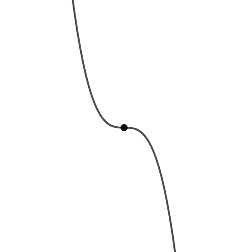
There are three types of stationary points - local minimums, local maximums and stationary point of inflections. Images of each stationary point is below.
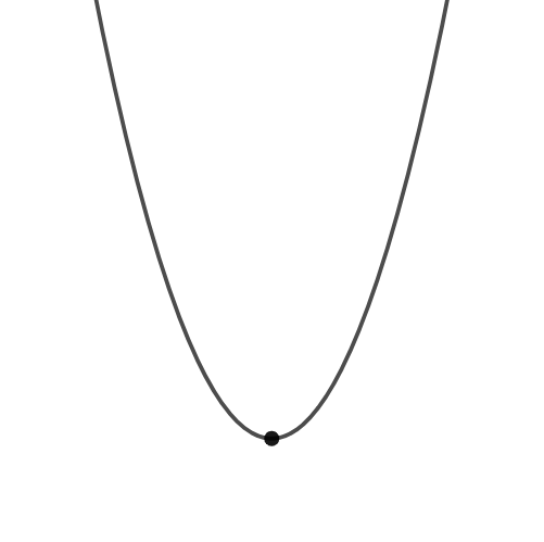
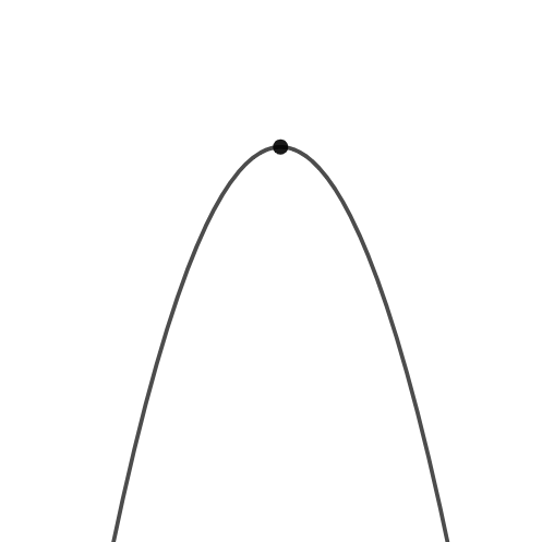
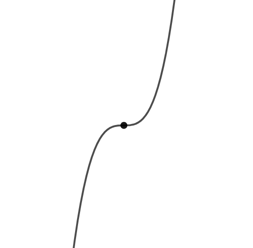
Here, we will detail the process for finding the coordinates of all the stationary points.
| 1 | Find f ’(x) |
| 2 | Solve f ’(x) = 0 for x |
| 3 | Substitute the x values found in step 2 into f(x) to find their corresponding y-coordinates. |
\[ \text{Example 7.6: Find the coordinates of the stationary points of the function } f(x) = x^4 - 6x^2 + 8x. \\ \text{ }\\ \begin{aligned} f(x) &= x^4 -6x^2 +8x \\ f’(x) &= 4x^3 - 12x + 8 \\ \text{Let } f’(x) &= 0 \\ 0 &= 4x^3 - 12x + 8 \\ &= 4(x-1)^2(x+2) \\ x &=-2, 1\\ f(-2) &= (-2)^4 - 6 \cdot (-2)^2 + 8 \cdot (-2) \\ f(-2) &= 16 - 24 -16 \\ f(-2) &= -24 \\ f(1) &= 1^4 - 6 \cdot 1^2 + 8 \cdot 1 \\ f(1) &= 1 - 6 + 8 \\ f(1) &= 3 \\ \end{aligned}\\ \text{ }\\ \text{The coordinates of the stationary points are: } (-2, -24) , (1,3) \\ \]
Having found the coordinates of the stationary point, we often want to know what sort of stationary point exists - local maximum, local minimum or a stationary point of inflection.
Finding the nature of the stationary point at x = b for the equation y = f(x).
| 1 | Find f ’(x) |
| 2 | Solve f ’(x) = 0 for x |
| 3 | Pick a ‘nice’, ‘round’ number (we will call this a) which is smaller than b, but larger than the x-coordinate of the next stationary point and inside the domain of the function. Also pick a ‘nice’, ‘round’ number (we will call this c) which is larger than b, but smaller than the x-coordinate of the next stationary point and inside the domain of the function. |
| 4 | Complete the following table: |
| 5 | Match the shape produced in the table to the corresponding stationary point. |
| x-coordinate | \[a\] | \[b\] | \[c\] |
| Gradient | \[f’(a)\] | \[0\] | \[f’(c)\] |
| Shape | \[\setminus \text{ or } /\] | \[-\] | \[\setminus\text{ or } /\] |
\[ \text{Example 7.7: State the nature of the stationary points of the function } f(x) = x^4 - 6x^2 + 8x. \\ \text{We have already found the stationary points in the section above, they are: } (-2, -24) \text{ and } (1,3). \\ \text{We will first find the nature of the stationary point: } (-2, -24) \\ \text{We will use } x = -3 \text{ as our point to the left of this stationary point and }\\ x= 0 \text{ as our point of this stationary point.} \\ \begin{aligned} f’(x) &= 4x^3 - 12x + 8 \\ f’(-3) &= 4 \cdot (-3)^3 -12 \cdot (-3) + 8 \\ f’(-3) &= -108 + 36 + 8\\ f’(-3) &= 64\\ f’(0) &= 4 \cdot 0^3 - 12 \cdot 0 + 8\\ f’(0) &= 8\\ \end{aligned}\\ \]
| \[\text{x-coordinate}\] | \[-3\] | \[-1\] | \[0\] |
| Gradient | \[64\] | \[0\] | \[8\] |
| Shape | \[\setminus\] | \[\_\] | \[/\] |
\[ \text{Thus, the point } (-2, -24) \text{ is a local minimum.}\\ \text{ } \\ \text{We will next find the nature of the other stationary point: } (1,3) \\ \text{We will use } x = 0 \text{ as our point to the left of this stationary point and }\\ x= 2 \text{ as our point of this stationary point.} \\ \begin{aligned} f’(x) &= 4x^3 - 12x + 8 \\ f’(0) &= 4 \cdot 0^3 - 12 \cdot 0 + 8\\ f’(0) &= 8\\ f’(2) &= 4 \cdot 2^3 - 12 \cdot 2 + 8 \\ f’(2) &= 32 - 24 + 8\\ f’(2) &= 16\\ \end{aligned}\\ \]
| \[\text{x-coordinate}\] | \[0\] | \[1\] | \[2\] |
| \[\text{Gradient}\] | \[8\] | \[0\] | \[16\] |
| \[\text{Shape}\] | \[/\] | \[\_\] | \[/\] |
\[\text{Thus, the point } (1, 3) \text{ is a stationary point of inflection.}\]
The standard exam two maximum/minimum problem goes something like this:
Someone is looking to build a fence around their farm to stop their cows from running away, but only has enough materials to make 5km worth of fencing. They wish to maximise the area of their field so that their beef can be classified as ‘free range’. Find the dimensions of the field which will allow them to do this and the corresponding area of the field.
Regardless of the story or functions provided, the system for finding the maximum/minimum of any function is the same.
| 1 | Identify (find) the equation of the function (let’s call it f(x)) which we want to calculate the maximum/minimum value for. This is very important. Often in a question there will be many functions, but you need to identify which function you want to know the maximum/minimum for. |
| 2 | Identify (find) the implied domain of f(x) |
| 3 | Find f ’(x) |
| 4 | Solve f ’(x) = 0 for x |
| 5 | Substitute the x values found in step 2 into f(x) to find their corresponding y-coordinates. Make sure that these stationary points are inside the domain of the function. |
| 6 | Substitute the endpoints of your domain into f(x) and find the corresponding y-coordinates. |
| 7 | Looking at all the y-values, state the maximum and/or minimum value of the function and whatever other information is required |
Note: Even if you are only asked for the maximum value, you must complete all steps which effectively means finding the minimum too.
\[ \text{Example 7.8: Find the maximum and minimum values of the function }\\ f \text{ and their corresponding } x \text{ values.} \\ f: [-2,5] \rightarrow \mathbb{R}, f(x) = x^3 -6x^2 +9x \\ \text{ }\\ \text{We will be finding the maximum/minimum values of } \\f(x) = x^3 -6x^2+9x \text{ which has domain } [-2,5] \\ \\ \begin{aligned} f’(x) &= 3x^2-12x + 9 \\ \text{Let } f’(x) &= 0 \\ 0 &= 3x^2 - 12x + 9 \\ &= x^2 - 4x + 3 \\ &= (x-3)(x-1) \\ x &= 1, 3 \\ \text{ }\\ f(1) &= 1^3 - 6 \cdot 1^2 + 9 \cdot 1 \\ f(1) &= 1 - 6 + 9 \\ f(1) &= 4 \\ f(3) &= 3^3 - 6 \cdot 3^2 + 9 \cdot 3 \\ f(3) &= 27 - 54 + 27 \\ f(3) &= 0 \\ f(-2) &= (-2)^3 - 6 \cdot (-2)^2 + 9 \cdot (-2) \\ f(-2) &= -8 - 24 - 18 \\ f(-2) &= -50 \\ f(5) &= 5^3 - 6 \cdot 5 ^2 + 9 \cdot 5 \\ f(5) &= 125 - 150 + 45 \\ f(5) &= 20 \\ \end{aligned}\\ \text{}\\ \text{Thus, the maximum value is 20 and occurs at } x = 5 \\ \text{ and the minimum value is -50 and occurs at } x = -2 \]