VCEMethods


Discrete Probability
The outcome of a random experiment is uncertain, but there exists a set of possible outcomes, \(\varepsilon\), known as the sample space.
The sum of the probabilities of all the outcomes in, \(\varepsilon\) is 1.
For example, the sample space for rolling a six-sided dice is:
\[\varepsilon = \{1,2,3,4,5,6\}\]
An event is a subset of the sample space denoted by a capital letter.
For example, if the event A is defined as the odd numbers when rolling a sixes sided dice, then we have:
\[A = \{1,3,5\}\]
If the event B is impossible, \(\text{Pr}\)(B) = 0. If the event B is certain, \(\text{Pr}\)(B) = 1. So, for any event B, 0 \(\leqslant\) \(\text{Pr}\)(B) \(\leqslant\) 1.
When the sample space is finite, the probability of an event is the sum of the probabilities of the outcomes in that event.
For example, if A is defined as the odd numbers when rolling a six sided dice, then:
\[ \begin{aligned} \Pr(A) &= \Pr(\text{Roll 1}) + \Pr(\text{Roll 3}) + \Pr(\text{Roll 5})\\ &= \frac{1}{6} + \frac{1}{6} + \frac{1}{6}\\ &= \frac{3}{6}\\ &= \frac{1}{2}\\ \end{aligned}\\ \]
When dealing with area questions, assume that it is equally likely to hit any region of the define area. So, the probability of hitting a certain region A is:
\[\text{Pr}(A) = \frac{\text{Area of A}}{\text{Total area}}\]
When an experiment has only two possible outcomes (events), they are said to be complementary. The complement of the event A is denoted by A'.
In the example with the six sided dice above, A' would represent everything in the sample space, except the odd numbers. So,
\[A' = \{2,4,6\}\]
Because the sum of the probabilities of events A and A' must be 1, we have:
\[\text{Pr}(A') = 1 - \text{Pr}(A)\]
The addition rule is generally used to calculate \(\Pr(A \cap B)\) or \(\Pr(A \cup B)\)
\[\Pr(A) + \Pr(B) - \Pr(A \cap B) = \Pr(A \cup B)\]
We say that two events are mutually exclusive if:
\[\Pr(A \cap B) = 0\]
That is the two events will never occur at the same time.
A very powerful table which isn't emphasised enough!
| \[A\] | \[A'\] | ||
| \[B\] | \[\Pr(A \cap B)\] | \[\Pr(A' \cap B)\] | \[\Pr(B)\] |
| \[B’\] | \[\Pr(A \cap B’)\] | \[\Pr(A' \cap B’)\] | \[\Pr(B’)\] |
| \[\Pr(A)\] | \[\Pr(A')\] | \[1\] |
For appropriate questions, place the probabilities given in their corresponding box. The sum of each column and row is the last entry. For example: \[\Pr(A \cap B) + \Pr(A \cap B') = \Pr(A)\]
\[ \text{Example 9.1: John has lost his class timetable. The probability that}\\\text{ he will have Methods period one is 0.35.}\\ \text{The probability that he has PE on a given day is 0.1 and the probability}\\ \text{ that he will have Methods period one and PE on the same day is 0.05.}\\ \text{Find the probability that John does not have Methods period one and PE on the same day.}\\ \text{ }\\ \text{Let } M \text{ represent methods period one and } P \text{ represent PE. From the information given we have:}\\ \]
| \[M\] | \[M’\] | ||
| \[P\] | \[0.05\] | \[\Pr(M’ \cap P)\] | \[0.1\] |
| \[P’\] | \[\Pr(M \cap P’)\] | \[\Pr(M’ \cap P’)\] | \[\Pr(P’)\] |
| \[0.35\] | \[\Pr(M’)\] | \[1\] |
\[ \text{Looking at the second row}\\ \begin{aligned} 0.05 + \Pr(M’ \cap P) &= 0.1\\ \Pr(M’ \cap P) &= 0.05\\ \text{} \\ \text{Looking at the last row}\\ 0.35 + \Pr(M’) &= 1\\ \Pr(M’) &= 0.65\\ \end{aligned} \]
| \[M\] | \[M’\] | ||
| \[P\] | \[0.05\] | \[0.05\] | \[0.1\] |
| \[P’\] | \[\Pr(M \cap P’)\] | \[\Pr(M’ \cap P’)\] | \[\Pr(P’)\] |
| \[0.35\] | \[0.65\] | \[1\] |
\[ \text{Looking at the third column}\\ \begin{aligned} 0.05 + \Pr(M’ \cap P’) &= 0.65\\ \Pr(M’ \cap P’) &= 0.6\\ \end{aligned}\\ \text{So, the probability that John does not have Methods period one and PE on a given day is } 0.6\\ \]
The probability that event A happens when we know that event B has already occured: \[\Pr(A \mid B) = \frac{\Pr(A \cap B)}{\Pr(B)}\]
It is often difficult to recognise when we are being asked a conditional probability question. However, generally speaking, if the question includes “if” or “given that”, you can be almost certain that you are dealing with conditional probability. We have written the same question below twice using the two different phrases.
\[ \text{Example 9.2 Find the probability that a six is rolled with a} \\\text{ six sided die given that an even number has been rolled. }\\ \text{Or equivelantly, If an even number has been rolled on a six sided die}\\\text{ find the probability that a six is rolled. }\\ \text{ }\\ \begin{aligned} \Pr(\text{Even}) &= \frac{3}{6} \\ \Pr(\text{Even and Six}) &= \Pr(\text{Six}) \\ &= \frac{1}{6} \\ \Pr(\text{Six if Even}) &= \frac{\Pr(\text{Even and Six})}{\Pr(\text{Even})} \\ &= \frac{\frac{1}{6}}{\frac{3}{6}}\\ &= \frac{1}{3}\\ \end{aligned}\\ \]
If knowing that event B has happened does not change the probability of event A from happening, then we say that events A and B are independent. For example, it raining outside and you going to school is independent as you will go to school regardless of whether it is raining or not. However, you being in class and having lunch is not independent as you will (probably) not be able to have lunch during class. Mathematically two events are independent if: \[ \begin{aligned} \Pr(A \cap B) &= \Pr(A) \cdot \Pr(B)\\ \Pr(A) \neq 0 &\text{ and } \Pr(B) \neq 0 \end{aligned} \]
\[ \text{Example 9.3: John has lost his class timetable.}\\\text{ The probability that he will have Methods period one is 0.35.}\\ \text{The probability that he has PE on a given day is 0.1 and the probability} \\\text{that he will have Methods period one and PE on the same day is 0.035.}\\ \text{Is John having Methods period one independent to him having PE on the same day?}\\ \text{ } \\ \text{A. Let } M \text{ represent methods period one and } P \text{ represent PE. From the information given we have:}\\ \begin{aligned} \Pr(M) &= 0.35\\ \Pr(P) &= 0.1\\ \Pr(M) \cdot \Pr(P) &= 0.035 \\ &= \Pr(M \cap P) \\ \end{aligned}\\ \text{So, John having Methods period one and PE on the same day are independent events} \\ \]
A random variable is a function that assigns a number to each outcome of an experiment.
A discrete random variable can take one of a countable number of possible outcomes. Continuous random variables will be considered in the next section.
For example, the number of free throws John can score when taking two is a discrete random variable which may take one of the values 0,1 or 2.
More on this below.
The probability distribution for a random variable consists of all the values the variable can take along with the associated probabilities. The general format is:
| \[\text{}\] | \[x_1\] | \[x_2\] | \[...\] | \[x_n\] |
| \[\Pr(X=x)\] | \[\Pr(X=x_1)\] | \[\Pr(X=x_2)\] | \[...\] | \[\Pr(X=x_n)\] |
The table allows us to easily find probabilities such as:
\(\text{Pr}(X>1)\) and \(\text{Pr}(X<2)\) by summing the relevant probabilities in the table
Note: the bottom row must sum to 1 and each probability must be at least zero and at most one.
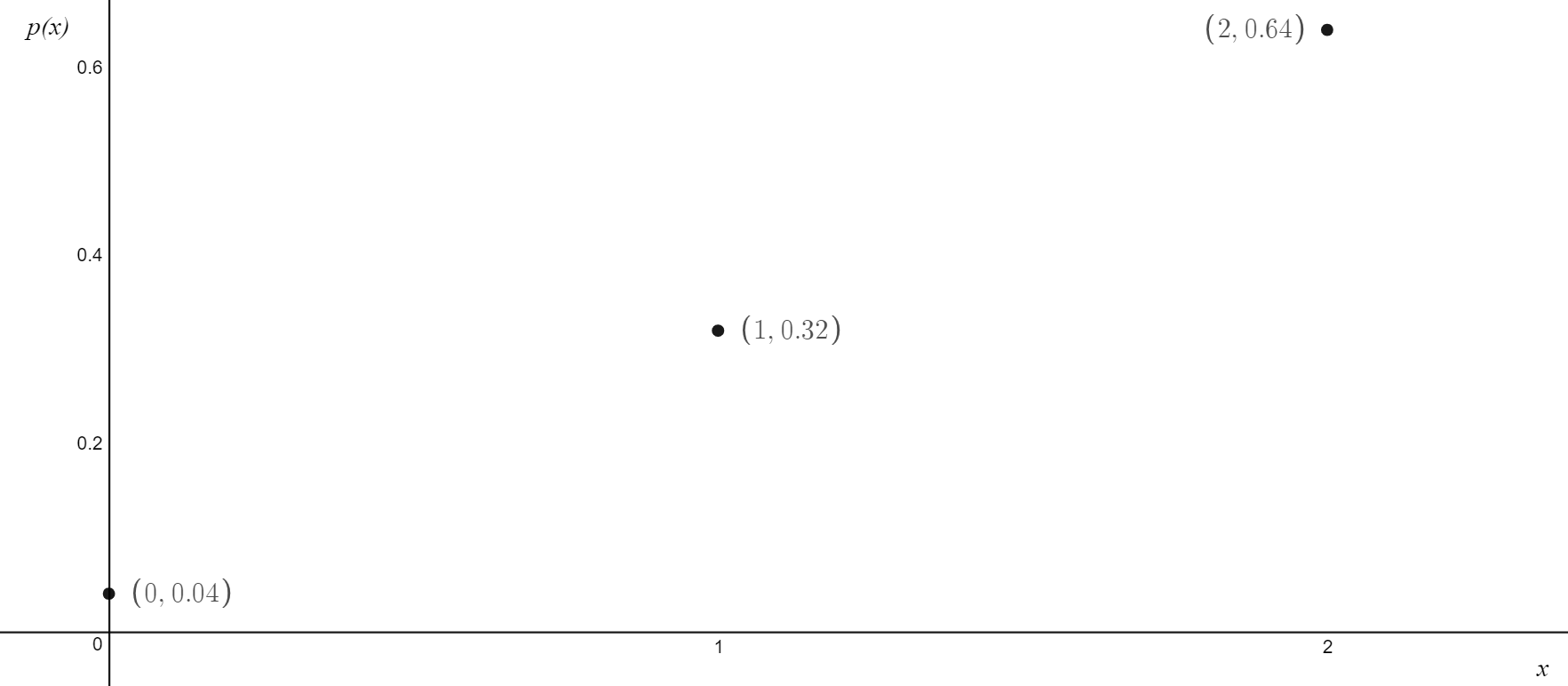
A discrete probability function, also called a probability mass function describes the distributions of a discrete random variable. An example of a graph for a discrete probability function is given below.
\[ \text{Example 9.4: James scores 80\% of all free throws he takes.}\\ \text{Create a probability distribution table and graph the probability mass function if James has two free throws.}\\ \text{ }\\ \text{Let } X \text{ be the number of free throws James scores}\\ \begin{aligned} \varepsilon &= {0,1,2}\\ Pr(X = 2) &= 0.80 \cdot 0.80 \\ &= 0.64\\ Pr(X = 1) &= \binom{2}{1} \cdot 0.8 \cdot 0.2\\ &= 0.32\\ Pr(X = 0) &= 0.2 \cdot 0.2 \\ &=0.04\\ \text{ }\\ \end{aligned}\\ \text{Bear with us on how we calculated } \Pr(X = 1). \\ \text{We will explain how we calculated this in the next chapter - binomial distribution}\\ \]
| \[x\] | \[0\] | \[1\] | \[2\] |
| \[\Pr(X=x)\] | \[0.04\] | \[0.32\] | \[0.64\] |
The expected value, or mean, is the average value of a discrete random variable. To calculate it, we sum the products of each value of X and its associated probability. That is, we first find the product of each column of the probability distribution table and then sum them up. Mathematically: \[E(X) = \mu = \sum_{x} x \cdot \Pr(x)\]
Variance and standard deviation are a measure of spread. Standard deviation is more relevant to us as it is in the same units as those which we are measuring. The formula provided by VCAA involves a very large number of calculations, as such we recommend you memorising: \[\text{Var}(X) = E(X^2) - [E(X)]^2\] To calculate the first term, simply square all of the x values in the top row of the probability distribution table and then find the product of each column of the probability distribution table before summing them up.
To get standard deviation we simply square root the variance. \[\text{sd}(X) = \sigma = \sqrt{\text{Var}(X)}\]
\[ \text{Note:}\\ \begin{aligned} E(aX+b) &= a \cdot E(X) + b\\ \text{Var}(aX+b) &= a^2 \cdot Var(X)\\ \end{aligned} \]
For many random variables, there is a 95% chance of obtaining an outcome within two standard deviations either side of the mean. That is, \[\Pr(\mu - 2\sigma \leqslant X \leqslant \mu + 2\sigma) \approx 0.95\]
\[ \text{Example 9.5: James scores 80\% of all free throws he takes. James takes two shots.}\\ \text{Find the expected value, variance and standard deviation for this scenario.}\\ \text{Correct your answers to 2 decimal points where appropriate}\\ \text{ }\\ \text{The probabilities for each outcome was calculated in example 9.3.}\\ \text{Let } X \text{ be the number of free throws James scores.}\\ \text{ }\\ \begin{aligned} E(X) &= 0 \times 0.04 + 1 \times 0.32 + 2 \times 0.64\\ &= 0 + 0.32 + 1.28\\ &= 1.6\\ \text{ }\\ E(X^2) &= 0^2 \times 0.04 + 1^2 \times 0.32 + 2^2 \times 0.64\\ &= 2.88\\ \text{ }\\ \text{Var}(X) &= E(x^2) - [E(X)]^2\\ &= 2.88 - 1.6^2\\ &= 0.32\\ \text{ }\\ \text{sd}(X) &= \sqrt{Var(X)}\\ \text{sd}(X) &= 0.57\\ \end{aligned} \]