VCEMethods


Exponential and Logs
Exponentials are comprised of a base and exponent (index or power). The general form is: \[A \cdot e^{nx + b} +c\]
A and n dilate the function
b and c translate the function
We refer to e as the base and nx + b collectively as the exponent
The basic shape of an exponential graph is shown below
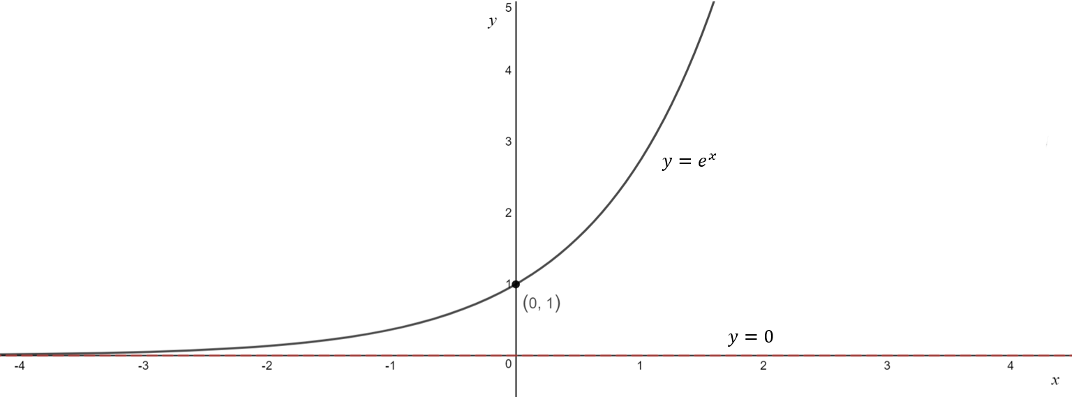
In general, unless told not to, all graphs must provide the coordinates or equations of any: x-intercepts, y-intercepts and asymptotes.
All exponential functions are presented in a manner somewhat similar to:
\[y = A \cdot e^{nx + b}+c\]
| 1 | Asymptote lies at y = c |
| 2 | Substitute x = 0 into the equation and solve for y to find the y-intercept |
| 3 | Substitute y = 0 into the equation and solve for y to find the x-intercept (not all exponentials will have one). |
| 4 | Connect the dots appropriately. Note that the graph must approach the asymptote at one end |
| 5 | Adjust the graph according to the domain, finding the coordinates of the endpoints if required. Label with the equation. |
\[
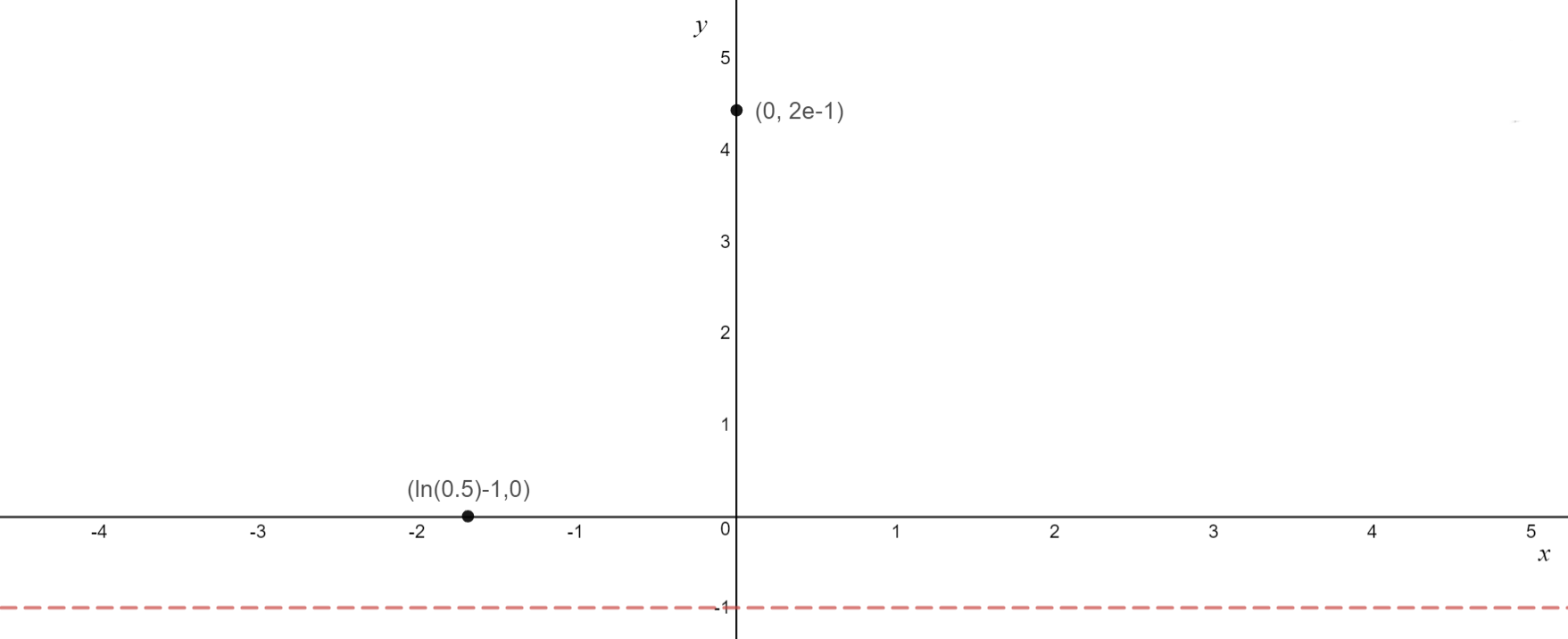
\text{Example 5.1: Sketch } y = 2e^{x+1}-1 \text{ labelling any x-intercepts and y-intercepts with} \\ \text{ their coordinates and asymptotes with their equations.}
\]
\[
\text{ } \\
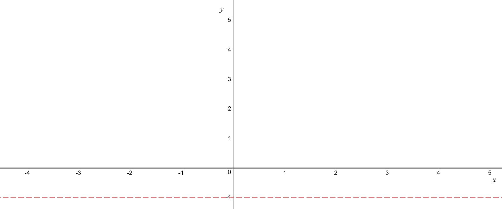
\text{1. Sketch in the asymptote} \\
\text{The asymptote lies at } y = -1
\]
\[
\text{ }\\
\text{2. Find the y-intercepts} \\
\begin{aligned}
x &= 0 \\
y &= 2e^{0 + 1} -1 \\
y &= 2e^{1} -1 \\
y &< 2 \cdot 3^{1} - 1 \\
y &< 5
\end{aligned}\\
\text{ }\\
\text{As we overestimated } e \text{ the y-intercept will lie be less than } 5\\
\]

\[
\text{ } \\
\text{3. Find the x-intercepts} \\
\begin{aligned}
y &= 0 \\
0 &= 2e^{x+1}-1 \\
\frac{1}{2} &= e^{x+1} \\
\log_{e}{\frac{1}{2}} &= x + 1 \\
\log_{e}{\frac{1}{2}} - 1 &= x \\
x &\approx -1.7 \text{ (CAS)} \\
\end{aligned} \\
\text{ }\\
\text{Read logarithms for more information on this calculation}
\]
\[
\text{ } \\
\text{4. Find the y-coordinate at } x=1 \\
\text{This step can be skipped as we have already found two points.}\\
\text{However, if you are not confident, there is no harm in finding an extra point.}
\]
\[
\text{ } \\
\text{5. Connect the dots}
\]

\[
\text{ } \\
\text{6. Adjust for the domain}\\
\text{No domain is provided. So we should use the implied domain. No changes required.}
\]
Euler’s number is denoted by the letter e and is irrational.
\[
\begin{aligned}
e &= \lim_{n\to \infty}(1+\frac{1}{n})^n\\
&\approx 2.718…\\
\end{aligned}\\
\]
e is just some random number.
You do not need to memorise what it equals!
| \[a^m \cdot a^n = a^{m+n}\] | \[\frac{a^m}{a^n} = a^{m-n}\] |
| \[(a^m)^n =a^{mn}\] | \[(ab)^n = a^n \cdot a^m\] |
| \[(\frac{a}{b})^n = \frac{a^n}{b^n}\] | \[a^0= 1\] |
| \[a^{-x}= \frac{1}{a^x}\] | \[a^{\frac{p}{q}} = (\sqrt[q]{a})^p = \sqrt[q]{a^p}\] |
Exponentials can only be manipulated when their bases are the same. Thus, when solving exponential equations it is necessary to try and change the bases of all (most) terms to the same thing.
\[
\text{Sample Questions: }\\
\text{Solve for }x:\\
\text{ }\\
\begin{aligned}
\text{Example 5.2: }7^x \times 49^{x+1} &= \frac{1}{7}\\
\text{ }\\
7^x \times 49^{x+1} &= \frac{1}{7} \\
7^x \times 7^{2^{x+1}} &= 7^{-1} \\
7^x \times 7^{2x+2} &= 7^{-1} \\
7^{x+2x+2} &= 7^{-1} \\
7^{3x+2} &= 7^{-1} \\
3x + 2 &= -1 \\
3x &= -3 \\
x &= -1 \\
\end{aligned}
\]
\[
\begin{aligned}
\text{Example 5.3: }\frac{2^{x^2-4}}{8^x}&=1\\
\text{ }\\
\frac{2^{x^{2}-4}}{8^x} &=1 \\
\frac{2^{x^{2}-4}}{2^{3^x}} &= 2^0) \\
\frac{2^{x^{2}-4}}{2^{3x}} &= 2^0) \\
2^{x^{2}-4-3x} &= 2^0 \\
x^2-3x-4 &= 0 \\
(x-4)(x+1) &= 0 \\
\end{aligned}\\
x=-1, x = 4
\]
\[
\begin{aligned}
\text{Example 5.4: }2(9^x) - 5(3^x) &= 3\\
\text{ }\\
2(9^x) -5(3^x) &= 3 \\
2(3^{2^x}) - 5(3^x) &= 3 \\
2(3^{x^2}) - 5(3^x) &= 3 \\
\text{Let } A &= 3^x \\
2A^2 - 5A &= 3 \\
2A^2 - 5A - 3 &= 0 \\
(2A +1)(A - 3) &= 0 \\
A = 3,\, A &= -\frac{1}{2} \\
3^x = 3,\,3^x &= -\frac{1}{2} \\
3^x &= -\frac{1}{2} \text{ is rejected as exponentials are positive} \\
3^x &= 3 \\
x &= 1\\
\end{aligned}\\
\]
\[
\begin{aligned}
\text{Example 5.5: }e^x &= 6 - 8e^{-x}\\
\text{ }\\
e^x &=6 - 8e^-x \\
e^x \cdot (e^x) &= e^x \cdot (6 - 8e^-x) \\
e^{2x} &= 6e^x - 8 \\
e^{x^2} &= 6e^x - 8 \\
\text{Let } A &= e^x \\
A^2 &= 6A - 8\\
A^2 - 6A + 8 &= 0\\
(A-4)(A-2) &= 0 \\
A = 4,& A = 2\\
e^x = 4,\,& e^x = 2\\
x=\log_{e}{4},\,& \log_{e}{2}\\
\end{aligned}\\
\text{ }\\
\text{ We will discuss the last step in the logarithm section below.}\\
\]
Logarithms are the inverse of exponentials. They have the general form: \[A \log_{e}{(nx + b)} + c\]
A and n dilate the function
b and c translate the function
We refer to e as the base
When evaluating a logarithm for example: \[\log_{a}{y}\] We want to think: what power must we take a to get y. Or symbolically: \[a^{\text{WHAT}} = y\]
Note that \(\log_{e}{x} = ln(x) \)
The basic shape of a logarithmic graph is shown below
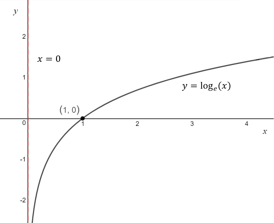
In general, unless told not to, all graphs must provide the coordinates or equations of any: x-intercepts, y-intercepts and asymptotes.
All logarithmic functions are presented in a manner somewhat similar to:
\[y = A\log_{e}{(nx + b)}+c\]
| 1 | Solve nx + b = 0 for x, this gives us the equation of the asymptote |
| 2 | Substitute y = 0 into the equation and solve for y to find the x-intercept |
| 3 | Substitute x = 0 into the equation and solve for y to find the y-intercept. (Not all logarithms have a y-intercept) |
| 4 | Let the argument (expression inside the log) equal to the base of the logarithm and solve for x and evaluate the function. (u,v) (u is the value of x just calculated and v the corresponding y-coordinate just calculated). |
| 5 | Connect the dots appropriately. Note that the graph must approach the asymptote at one end |
| 6 | Adjust the graph according to the domain, finding the coordinates of the endpoints if required. |
\[
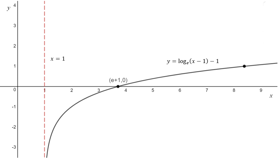
\text{Example 5.5: Sketch } y = \log_{e}{(x-1)} -1 \text{ labelling any x-intercepts and y-intercepts with} \\ \text{ their coordinates and asymptotes with their equations.}
\]
\[
\text{ } \\
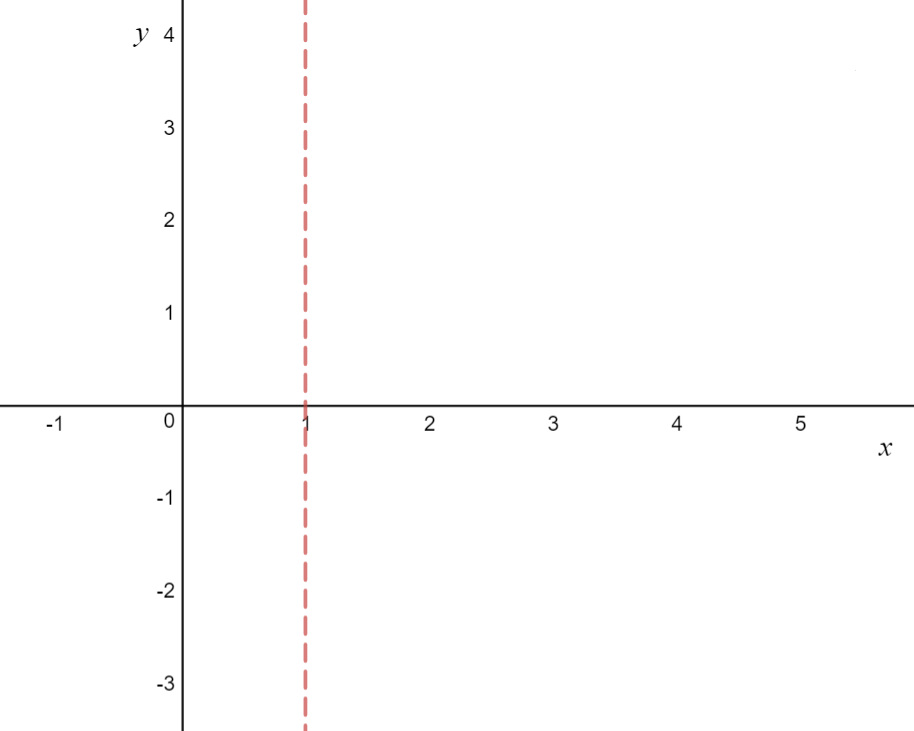
\text{1. Sketch in the asymptote} \\
\begin{aligned}
x-1&= 0\\
x &= 1\\
\end{aligned}
\]
\[
\text{ } \\
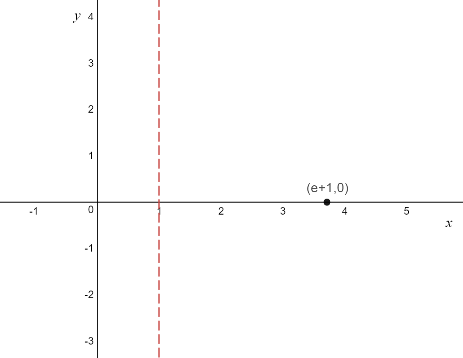
\text{2. Find the x-intercepts} \\
\begin{aligned}
y&=0\\
0&=\log_{e}{(x-1)}-1\\
1&=\log_{e}{(x-1)} \\
e^{1} &= x-1 \\
e + 1 &= x \\
3 + 1 &\approx x \\
4 &\approx x \\
\end{aligned}\\
\text{As we overestimated } e \text{ the x-intercept will lie between } 3 \text{ and } 4
\]
\[
\text{ } \\
\text{3. Find the y-intercepts} \\
\text{There will be no y-intercepts.} \\
\text{The x-intercept is to the right of the asymptote and the asymptote is to the right of the y-axis} \\
\text{It is therefore impossible for the graph to have a y-intercept}
\]
\[
\text{ } \\
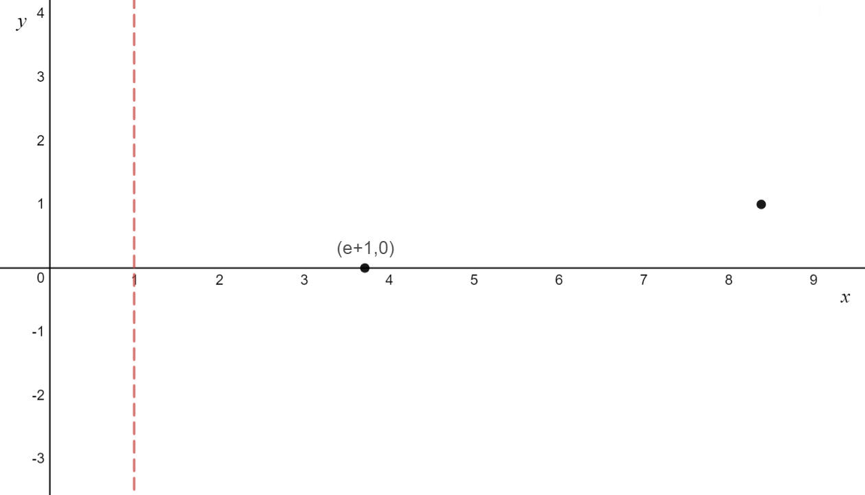
\text{4. Find an additional point} \\
\text{The base of the logarithm is } e \\
\text{We will set the argument of the logarithm be equal to } e \\
\text{ }\\
\begin{aligned}
x-1&=e \\
x&=e+1 \\
\end{aligned}\\
\text{ }\\
x=e+1 \text{ is the x-intercept. Let’s find another point. }\\
\text{We will set the argument of the logarithm be equal to } e^2 \\
\text{ }\\
\begin{aligned}
x-1&=e^2 \\
x&=e^2+1 \\
y&=\log_{e}{(e^2+1-1)}-1 \\
y&=\log_{e}{e^2}-1 \\
y&=2-1 \\
y&=1
\end{aligned}\\
\]
\[
\text{ } \\
\text{5. Connect the dots}
\]
\[
\text{ } \\
\text{6. Adjust for the domain}\\
\text{No domain is provided. So we should use the implied domain. No changes required.}
\]
| \[a^x = y \Leftrightarrow \log_{a}{y} = x\] | \[\log_{a}{mn} = \log_{a}{m} + \log_{a}{n}\] |
| \[\log_{a}{\frac{m}{n}} = \log_{a}{m}-\log_{a}{n}\] | \[\log_{a}{\frac{1}{n}} = -\log_{a}{n}\] |
| \[\log_{a}{m^p} = p \cdot \log_a{m}\] | \[\log_{a}{a} = 1\] |
| \[\log_{a}{a^x} = x\] | \[a^{\log_{a}{x}} = x\] |
| \[\log_{a}{x} = \frac{\log_{b}{x}}{\log_{b}{a}}\] | \[a^x = b^{(\log_{b}{a}) \cdot x}\] |
Just like exponentials, logarithms can only be manipulated when their bases are the same. Thus, it is necessary to try and change the bases of all (most) terms to the same thing.
\[ \text{Solve the following for }x\\ \text{ }\\ \begin{aligned} \text{Example 5.6: } 2\log_{2}{x} - \log_{2}{x^3} &= 5\\ \text{ }\\ 2\log_{2}{x}-\log_{2}{x^3} &= 5 \\ \log_{2}{x^2}-\log_{2}{x^3} &= 5 \\ \log_{2}{\frac{x^2}{x^3}}&= 5 \\ \log_{2}{\frac{1}{x}}&= 5\\ \frac{1}{x} &= 2^5 \\ x &= \frac{1}{2^5} \\ x &= \frac{1}{32} \end{aligned} \] \[ \begin{aligned} \text{Example 5.7: }\log_{e}{(\frac{2}{x})} + 2\log_{e}{x} &= 1\\ \text{ }\\ \log_{e}{\frac{2}{x}} + 2\log_{e}{x} &= 1 \\ \log_{e}{\frac{2}{x}} + \log_{e}{x^2} &= 1 \\ \log_{e}{\frac{2x^2}{x}}&= 1 \\ \log_{e}{2x}&= 1 \\ e^1 &= 2x \\ \frac{e}{2} &= x\\ \end{aligned}\\ \] \[ \begin{aligned} \text{Example 5.8: }\log_{2}{6} &= 1 + \log_{4}{x}\\ \text{ }\\ \log_{2}{6} &= 1 + \log_{4}{x} \\ \frac{\log_{4}{6}}{\log_{4}{2}} &= 1 + \log_{4}{x} \\ \frac{\log_{4}{6}}{\log_{4}{2}} - 1 &= \log_{4}{x} \\ \frac{\log_{4}{6}}{\frac{1}{2}} - 1 &= \log_{4}{x} \\ 2\log_{4}{6} - \log_{4}{4} &= \log_{4}{x} \\ 2\log_{4}{6} - \log_{4}{4} &= \log_{4}{x} \\ \log_{4}{6^2} - \log_{4}{4} &= \log_{4}{x} \\ \log_{4}{\frac{6^2}{4}} &= \log_{4}{x} \\ \log_{4}{9} &= \log_{4}{x} \\ 9 &= x \\ \end{aligned}\\ \] \[ \text{Example 5.9: Re-write }2^x \text{ with } e \text{ as the base}\\ \text{ }\\ 2^x = e^{\log_{e}{(2^x)}}\\ \]
The general form of an exponential and logarithm is shown below. However, the question will always provide us with the form we should use, this means that the equation provided may or may not have as many unknowns as the ones below. \[y = Ae^{(nx + b)} + c\] \[y = A\log_{e}{(nx + b)}+c\]
\[ \text{For exponentials: The value of c will simply be the value of the horizontal asymptote. }\\ \text{ }\\ \text{For logarithms: The value of }-\frac{b}{n}\text{ will be the value of the vertical asymptote.}\\ \text{ }\\ \text{To find the value of any other unknowns, simply substitute the x and y-coordinates of any}\\ \text{ additional points provided into the equation}\\ \text{ (having found some unknowns as detailed above) and solve them (simultaneously).} \]
\[
\text{ }\\
\text{Example 5.9: The rule of the graph shown is the form } y = a\log_{3}{(x+b)}. \\ \text{ Find the values of } a \text{ and } b.
\]
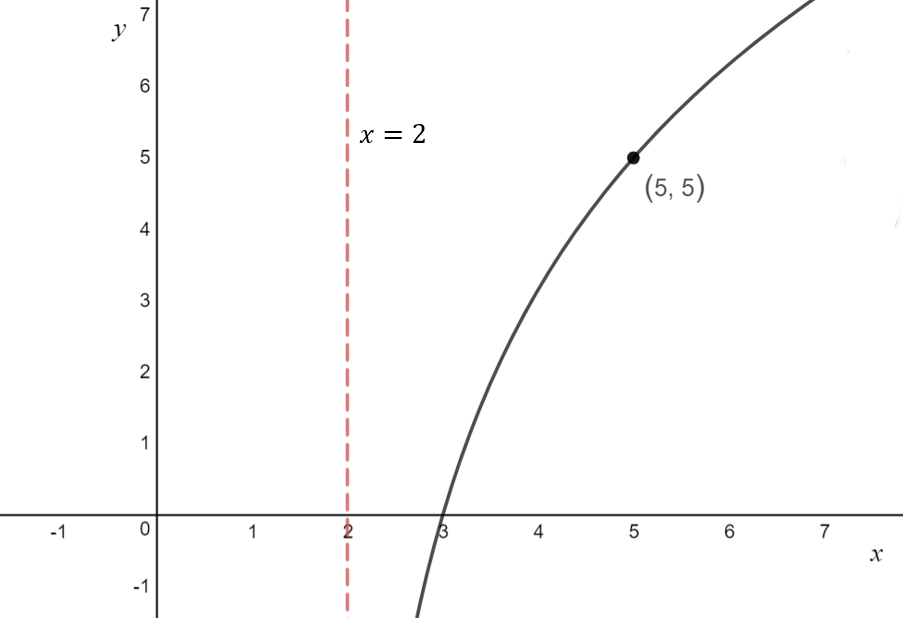
\[
\text{There is an asymptote at } x = 2 \\
\begin{aligned}
2+b&=0 \\
b&=-2 \\
y&=a\log_{3}{(x-2)} … \boxed{1} \\
\end{aligned}
\text{} \\
\text{Substitute } (5,5) \text{ into } \boxed{1} \\
\begin{aligned}
5 &= a\log_{3}{(5-2)} \\
5&=a\log_{3}{3} \\
5&= a \cdot 1 \\
5 &= a \\
\end{aligned}\\
a = 5, \, b = -2 \\
\]
\[
\text{Example 5.10: The rule of the graph shown is the form } y = ae^{-bx} \text{ Find the values of } a \text{ and } b.
\]
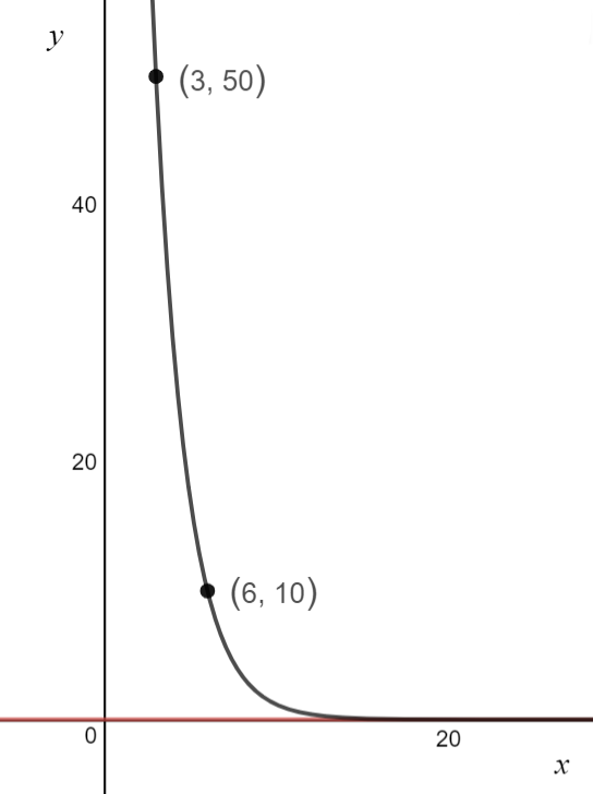
\[
\text{The equation of the asymptote has not been provided, however we have two points. }\\
\text{We have points } (3,50) \text{ and } (6,10) \\
\begin{aligned}
50 = ae^{-3b} … \boxed{1} \\
10 = ae^{-6b} …\boxed{2} \\
\boxed{1} &\div \boxed{2} \\
\frac{50}{10} &= \frac{ae^{-3b}}{ae^{-b}} \\
5 &= e^3b\\
\log_{e}{5} &= 3b \\
\frac{\log_{e}{5}}{3} &= b \\
\text{Substitute } b= &\frac{\log_{e}{5}}{3} \text{ into } \boxed{1} \\
50 &= ae^{-3 \cdot \frac{\log_{e}{5}}{3}} \\
50 &= ae^{-\log_{e}{5}} \\
50 &= ae^{\log_{e}{5^{-1}}} \\
50 &= a \cdot 5^{-1} \\
50 &= \frac{1}{5} a \\
250 &= a \\
\end{aligned}\\
a = 250, \, b = \frac{\log_{e}{5}}{3}\\
\]