VCEMethods


Normal Distribution
The normal distribution is a continuous probability distribution. It has the equation:
\[f(x) = \frac{1}{\sigma \sqrt{2\pi}}e^{-\frac{1}{2}(\frac{x-\mu}{\sigma})^2}\]
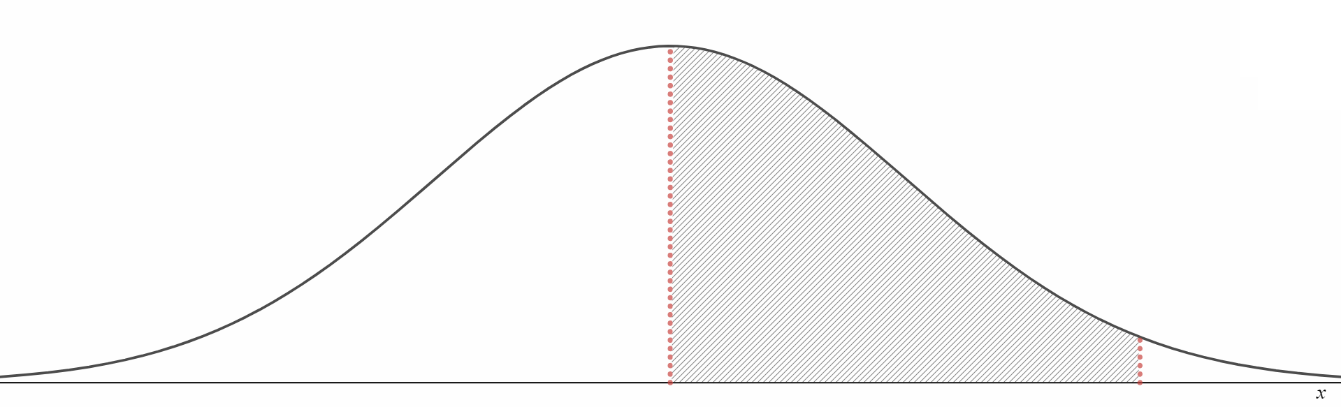
The graph of a normal distribution is symmetrical and bell shaped.
As with all probability density functions, the area under the curve is equal to one, and the probabilities correspond to the area under the curve.
Integrating the normal equation is beyond the scope of this course. We describe how to calculate probabilities below with a CAS calculator. Just with the binomial distribution, do not use calculator notation, simply show that you recognise that you are dealing with a normal distribution with: \[X \sim N(\mu, \sigma^2)\]
The standard normal distribution, Z, is the simplest form of the normal distribution. It has a mean of zero and standard deviation of one (and variance of one). \[Z \sim N(0,1)\] We will often refer back to the standard normal distribution when solving problems.
To compare results on different normal distributions (for example results of a VCE student and IB student) it is convenient to convert all values to the standard normal distribution.
The standard normal distribution as discussed above is:
\[Z \sim N(0,1)\]
For any normal distribution, \[X \sim N(\mu, \sigma^2)\] \[z = \frac{x - \mu}{\sigma} \text{ is the standardised value}\] \[\text{Thus, } \Pr(X \leqslant x) = \Pr(Z \leqslant \frac{x - \mu}{\sigma})\] This is true for any combination of inequality signs, simply replace the x value with the standardized value and change X into Z to indicate that we are now dealing with the standard normal distribution.
\[ \text{Example 12.1: Below are the test scores of three different students who took different tests.}\\\text{The test results in all three cases were normally distributed and}\\ \text{their respective means and standard deviations have been provided.}\\\text{ Rank the students from best to worst }\\ \]
| \[\text{Score}\] | \[\mu\] | \[\sigma\] | |
| \[\text{John}\] | 45 | 30 | 7 |
| \[\text{Amy}\] | 80 | 50 | 12 |
| \[\text{Bob}\] | 160 | 100 | 25 |
\[ \begin{aligned} z_{John} &= \frac{45-30}{7}\\ & \approx 2.14\\ \text{ }\\ z_{Amy} &= \frac{80 - 50}{12}\\ &= 2.5\\ \text{ }\\ z_{Bob} &= \frac{160-100}{25}\\ &= 2.4\\ \end{aligned} \text{ }\\ \text{ }\\ \text{Performance from best to worst - Amy, Bob and John}\\ \]
\[X \sim N(\mu, \sigma^2)\] \[\Pr(\mu-\sigma \leqslant X \leqslant \mu+\sigma) \approx 0.68\] \[\Pr(\mu-2\sigma \leqslant X \leqslant \mu+2\sigma) \approx 0.95\] \[\Pr(\mu-3\sigma \leqslant X \leqslant \mu+3\sigma) \approx 0.997\]
These are approximations and should only be used in exam one (unless indicated by the question).
Note that we are now able to find the probabilities for any combination of \(\mu - c \cdot \sigma ,\, c = \{1,2,3\}\) as the normal distribution is symmetrical about the line \(x = \mu\). An example is given below.
\[
\text{Example 12.2: } X \text{ is normal with } E(X) = 30 \text{ and } sd(X) = 7.\\ \text{ Find } \Pr(30 \leqslant X \leqslant 44) \text{ and } \Pr(X \geqslant 44). \text{ Use the } 68-95-99.7\% \text{ rule. }\\
\text{Almost all VCE subjects scores are normally distributed with } E(X) = 30 \text{ and } sd(X) =7. \\
\text{ }
\]
 \[
X \sim N(30, 7^2)\\
\begin{aligned}
44 &= \mu + 2\sigma\\
\Pr(\mu -2\sigma \leqslant X \leqslant \mu +2\sigma) &= 0.95\\
\Pr(\mu \leqslant X \leqslant \mu + 2\sigma) &= \frac{0.95}{2}\\
\Pr(30 \leqslant X \leqslant 44) &= 0.475\\
\end{aligned}\\
\text{ }\\
\]
\[
X \sim N(30, 7^2)\\
\begin{aligned}
44 &= \mu + 2\sigma\\
\Pr(\mu -2\sigma \leqslant X \leqslant \mu +2\sigma) &= 0.95\\
\Pr(\mu \leqslant X \leqslant \mu + 2\sigma) &= \frac{0.95}{2}\\
\Pr(30 \leqslant X \leqslant 44) &= 0.475\\
\end{aligned}\\
\text{ }\\
\]
 \[
\text{ } \\
\begin{aligned}
\Pr(\mu \leqslant X \leqslant \mu + 2\sigma) &= \frac{0.95}{2}\\
&= 0.475\\
\Pr(X \leqslant \mu) &= 0.5\\
\Pr(X \leqslant \mu + 2\sigma) &= \Pr(X \leqslant \mu) + \Pr(\mu \leqslant X \leqslant \mu + 2\sigma)\\
&= 0.475 + 0.5\\
&= 0.975\\
\Pr(X \geqslant \mu + 2\sigma) &= 1 - \Pr(X \leqslant \mu + 2\sigma)\\
&= 1 - 0.975\\
&= 0.025\\
\Pr(X \geqslant 44) &= 0.025\\
\end{aligned}\\
\]
\[
\text{ } \\
\begin{aligned}
\Pr(\mu \leqslant X \leqslant \mu + 2\sigma) &= \frac{0.95}{2}\\
&= 0.475\\
\Pr(X \leqslant \mu) &= 0.5\\
\Pr(X \leqslant \mu + 2\sigma) &= \Pr(X \leqslant \mu) + \Pr(\mu \leqslant X \leqslant \mu + 2\sigma)\\
&= 0.475 + 0.5\\
&= 0.975\\
\Pr(X \geqslant \mu + 2\sigma) &= 1 - \Pr(X \leqslant \mu + 2\sigma)\\
&= 1 - 0.975\\
&= 0.025\\
\Pr(X \geqslant 44) &= 0.025\\
\end{aligned}\\
\]
\[\text{Remember } \Pr(a \leqslant X \leqslant b) = \Pr(a < X \leqslant b) = \Pr(a \leqslant X < b) = \Pr(a < X < b)\] \[\text{To calculate } \Pr(a \leqslant X \leqslant b) \text{ use } normCdf(a,b,\mu,\sigma)\] \[\text{To calculate } \Pr(X \leqslant c) \text{ use } normCdf(-\infty,c,\mu,\sigma)\] \[\text{To calculate } \Pr(X \geqslant d) \text{ use } normCdf(d,\infty,\mu,\sigma)\] \[X \sim N(20, 5^2)\]
| Question | Calculator command | Answer (correct to 3 d.p) |
| \[\Pr(18 \leqslant X \leqslant 23)\] | \[normCdf(18, 23, 20, 5)\] | \[0.381\] |
| \[\Pr(X \leqslant 15)\] | \[normCdf(-\infty, 15, 20, 5)\] | \[0.159\] |
| \[\Pr(X \leqslant 22 \mid X \geqslant 20)\] | \[\frac{normCdf(20, 22,20,5)}{normCdf(20,\infty,20,5)}\] | \[0.311\] |
The inverse normal function on our CAS allows us to find the corresponding value of x when the probability (or area) is known. The inverse normal function always calculates the area which you provide it from the left hand side. Mathematically, the calculator is always looking to calculate c when you give it in the area: \[ \begin{aligned} \Pr(X < c) &= \text{Area} \\ c&= invNorm(\text{Area}, \,\mu, \,\sigma) \\ \end{aligned} \]
Thus, if we are not given a probability in the form above, we must use symmetry properties of the normal distribution to adjust the probability into the form above. All normal distributions are symmetrical about \(\mu\).
The table below shows you how to find the unknown c. We assume that the probability (Area) is given in the question.
| Expression | How to find c |
| \[\Pr(X \leqslant c) = p\] | \[c = invNorm(p,\, \mu,\, \sigma)\] |
| \[\Pr(X \geqslant c) = p\] | \[ \begin{aligned} \Pr(X \geqslant c) &= 1 - \Pr(X \leqslant c) \\ \Pr(X \geqslant c) &= 1 - p \\ \Pr(X \leqslant c) &= -(p - 1) \\ c &= invNorm(1 - p,\, \mu,\, \sigma)\\ \end{aligned} \] |
| \[\Pr(-c \leqslant X \leqslant c) = p\] | \[ \begin{aligned} \Pr(-c \leqslant X \leqslant c) &=1- 2\Pr(X \leqslant -c)\\ \Pr(X \leqslant -c) &= \frac{1-p}{2} \\ -c &= invNorm(\frac{1-p}{2}, \, \mu, \, \sigma)\\ c &= -invNorm(\frac{1-p}{2}, \, \mu, \, \sigma)\\ \end{aligned} \] |
All the examples below will use the standard normal distribution. However, as indicated above, you are able to enter different values for \(\mu\) and \(\sigma\).
\[
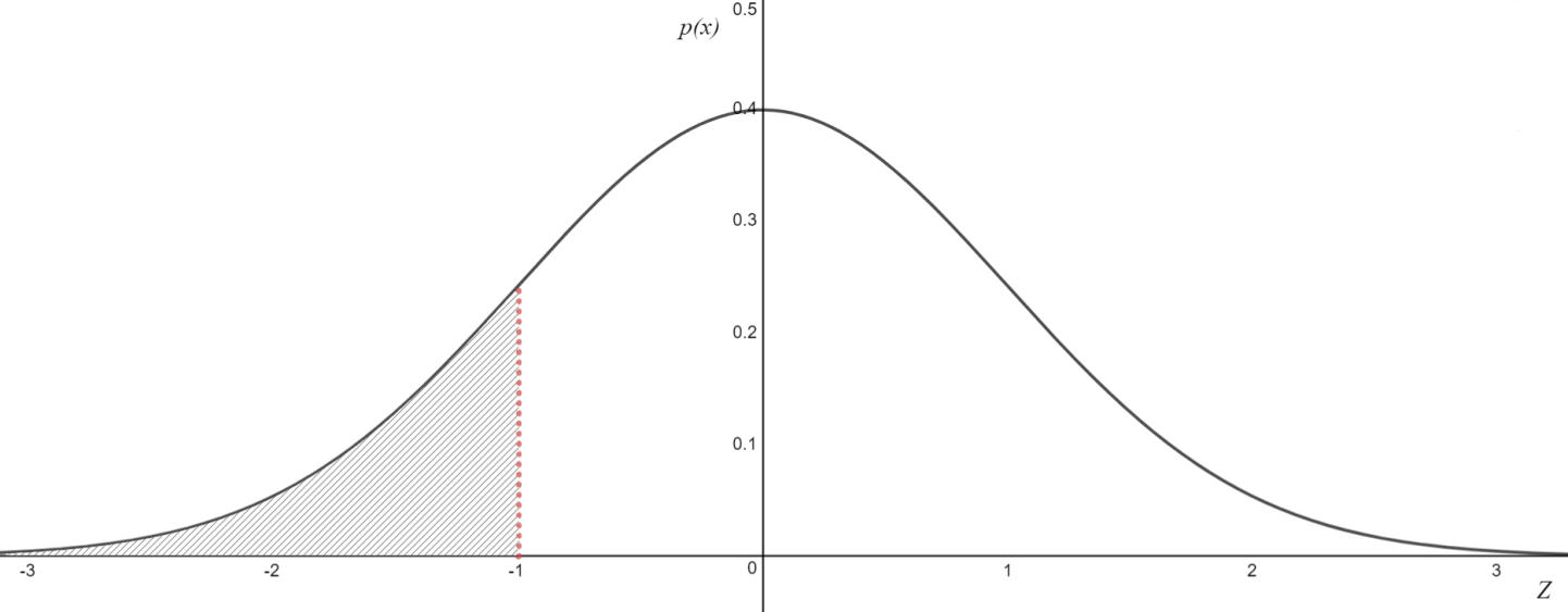
\text{Example 12.3: Find the value of }c, \text{ correcting to four decimal points, if } \Pr(Z < c) =0.16 \\
\text{ }
\]
 \[
\text{ } \\
\begin{aligned}
\Pr(Z < c) &= 0.16 \\
c &= invNorm(0.16, 0, 1) \\
c &= -0.9945\\
\end{aligned}
\]
\[
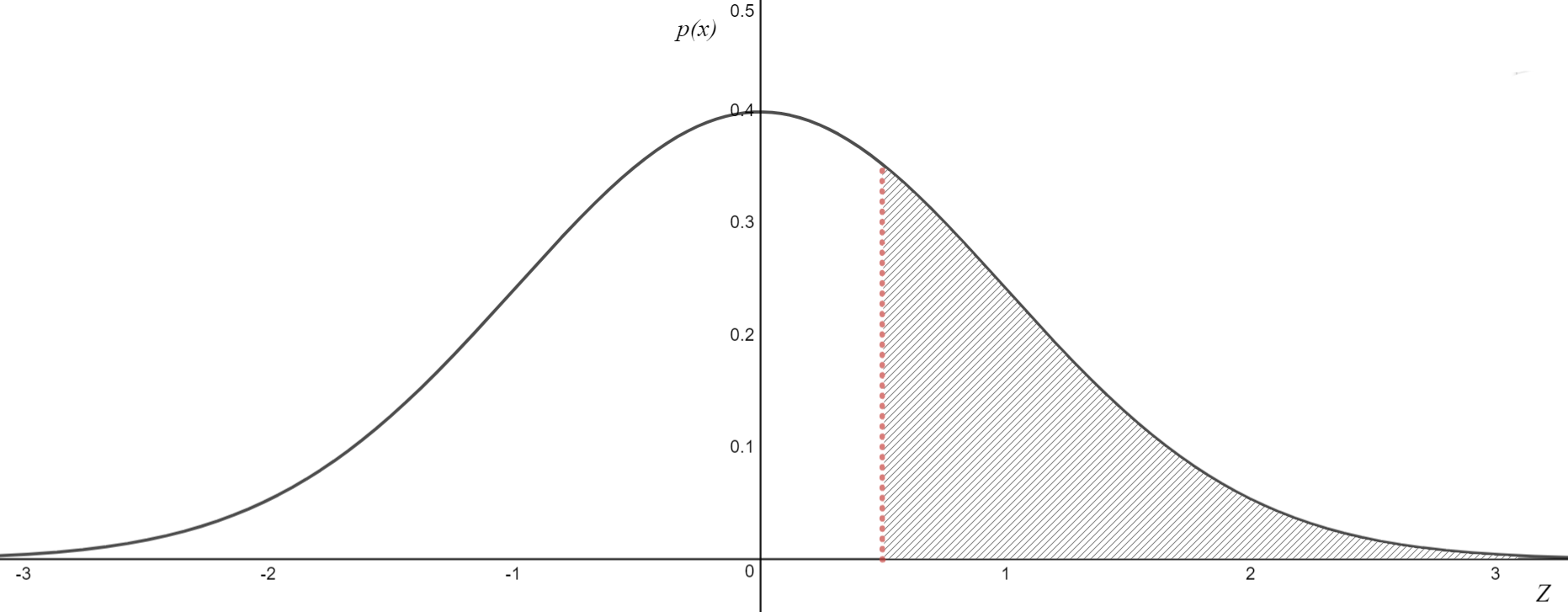
\text{Example 12.4: Find the value of }c, \text{ correcting to four decimal points, if } \Pr(Z > c) =0.33 \\
\text{ }
\]
\[
\text{ } \\
\begin{aligned}
\Pr(Z < c) &= 0.16 \\
c &= invNorm(0.16, 0, 1) \\
c &= -0.9945\\
\end{aligned}
\]
\[
\text{Example 12.4: Find the value of }c, \text{ correcting to four decimal points, if } \Pr(Z > c) =0.33 \\
\text{ }
\]
 \[
\text{ } \\
\begin{aligned}
\Pr(Z > c) &=0.33 \\
1-\Pr(Z >c) &= 1-0.33 \\
\Pr(Z < c) &= 0.67 \\
c&=invNorm(0.67, 0, 1) \\
c&=0.4400\\
\end{aligned}
\]
\[
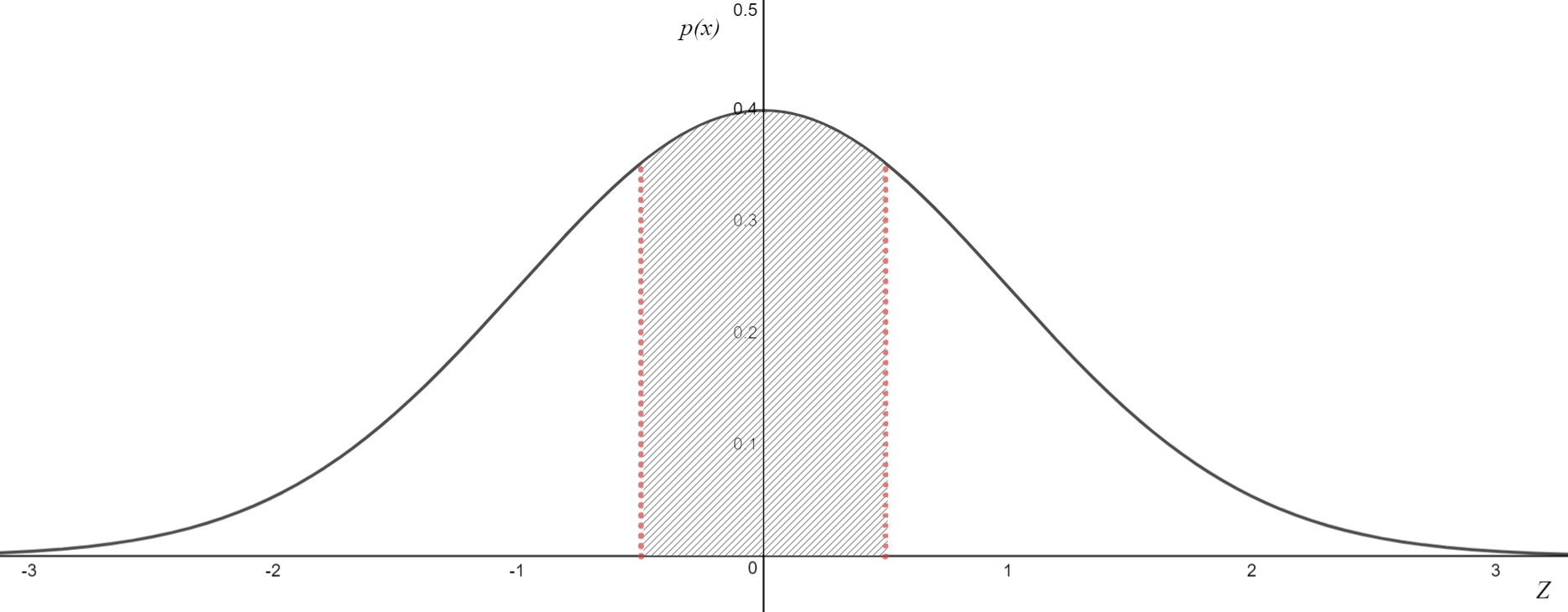
\text{Example 12.5: Find the value of }c, \text{ correcting to four decimal points, if } \Pr(-c < Z < c) =0.5 \\
\text{ }
\]
\[
\text{ } \\
\begin{aligned}
\Pr(Z > c) &=0.33 \\
1-\Pr(Z >c) &= 1-0.33 \\
\Pr(Z < c) &= 0.67 \\
c&=invNorm(0.67, 0, 1) \\
c&=0.4400\\
\end{aligned}
\]
\[
\text{Example 12.5: Find the value of }c, \text{ correcting to four decimal points, if } \Pr(-c < Z < c) =0.5 \\
\text{ }
\]
 \[
\text{ } \\
\begin{aligned}
\Pr(-c < Z < c) &=0.5 \\
1 - 2\Pr(Z < -c) &= 0.5 \\
-2\Pr(Z < -c) &= -0.5 \\
\Pr(Z < -c) &= 0.25 \\
-c &= invNorm(0.25, 0, 1) \\
-c &= -0.6745 \\
c &= 0.6745 \\
\end{aligned}
\]
\[
\text{ } \\
\begin{aligned}
\Pr(-c < Z < c) &=0.5 \\
1 - 2\Pr(Z < -c) &= 0.5 \\
-2\Pr(Z < -c) &= -0.5 \\
\Pr(Z < -c) &= 0.25 \\
-c &= invNorm(0.25, 0, 1) \\
-c &= -0.6745 \\
c &= 0.6745 \\
\end{aligned}
\]
Although the binomial distribution is discrete, it can be approximated by the normal distribution when the sample size is large enough. If both \(\mu\) and \(\sigma\) are greater than 5, the normal approximation can be used with reasonable accuracy.Only use the normal approximation for the binomial distribution if the question explicitly asks for it. This is very rare.
\[ \text{Example 12.6: Use the normal approximation to the binomial distribution to find the}\\\text{approximate probability, correct to 4 decimal places, that }\\ \text{in the next 600 rolls of a fair die, less than 120 sixes will be rolled}\\ \text{ }\\ \text{Let } X \text{ be the number of sixes rolled}\\ \begin{aligned} E(X) &= np\\ &= 600 \times \frac{1}{6}\\ &= 100\\ sd(X) &= \sqrt{np(1-p)}\\ &= \sqrt{100 \cdot (1 - \frac{1}{6})}\\ &= \sqrt{\frac{500}{6}}\\ \end{aligned}\\ \text{Using a normal approximation: }\\ X \sim N(100, (\sqrt{\frac{500}{6}})^2)\\ \begin{aligned} \Pr(X <120) &= nomCdf(0, 120, 100, \sqrt{\frac{500}{6}})\\ &= 0.9858\\ \end{aligned}\\ \]
This is a common, but harder question. An example is given below.
\[ \text{Example 12.7 The age of basketball players at a club is normally distributed. }\\ \text{If 10\% of players are under the age of 15 and 8\% are over the age of 20,}\\ \text{find the mean and standard deviation of the player’s ages correct to two decimal points}\\ \text{ }\\ \text{Let } X \text{ be the age of the basketball club members and } Z \text{ be the standard normal distribution.}\\ X \sim N(\mu, \sigma^2)\\ Z \sim N(0,1)\\ \text{ }\\ \begin{aligned} \Pr(X < 15) &= 0.1\\ \Pr(Z < \frac{15-\mu}{\sigma}) &= 0.1\\ \frac{15-\mu}{\sigma} &= invNorm(0.1,0,1)\\ \frac{15-\mu}{\sigma} &\approx -1.281… \,\boxed{1}\\ \text{ }\\ \Pr(X > 20) &= 0.08\\ \Pr (Z > \frac{20-\mu}{\sigma}) &= 0.08\\ \Pr (Z < \frac{20-\mu}{\sigma}) &= 1-0.08\\ \Pr (Z < \frac{20-\mu}{\sigma}) &= 0.92\\ \frac{20-\mu}{\sigma} &= invNorm(0.92, 0,1)\\ \frac{20-\mu}{\sigma}&\approx 1.405… \, \boxed{2}\\ \end{aligned}\\ \text{Solving } \boxed{1} \text{ and } \boxed{2} \text{ for } \mu \text{ and } \sigma\\ \begin{aligned} \mu &= 17.39\\ \sigma &= 1.86\\ \end{aligned}\\ \]